
13. Profile Hidden Markov Models#
13.1. Overview#
Profile Hidden Markov Models (HMMs) are statistical models designed to capture the variability and patterns found in multiple sequence alignments (MSAs). They offer a robust way to model conserved regions, sequence motifs, and evolutionary variations, making them an essential tool in bioinformatics for sequence analysis and comparison.
13.2. Profile HMMs as representations of MSAs#
A multiple sequence alignment of a homologous family of protein domains reveals patterns of site-specific evolutionary conservation:
Conserved Residues: Certain positions show high conservation, reflecting key functional or structural roles.
Substitution Patterns: Some positions tolerate substitutions that conserve physiochemical properties like hydrophobicity, charge, or size.
Variable Positions: Some positions exhibit near-neutral variability.
Insertions and Deletions: Insertions and deletions are tolerated at some positions more than others.
A profile HMM is a position-specific scoring model that describes which symbols are likely to be observed and how frequently insertions or deletions occur at each position (column) of a multiple sequence alignment.
Probabilistic Basis: HMMs have a formal probabilistic basis, allowing the use of probability theory to set and interpret the large number of free parameters in a profile, including position-specific gap and insertion parameters.
Automatable Methods: These methods are mathematically consistent and automatable, enabling the creation of libraries of hundreds of profile HMMs for large-scale genome analysis.
13.2.1. Applications#
Profile HMMs offer several key applications in bioinformatics:
Sequence Alignment: By comparing a new sequence to a profile HMM, we can identify which regions of the sequence correspond to conserved regions in the MSA, helping to align the new sequence with known homologs.
Domain Detection: Profile HMMs can identify and characterize functional domains in proteins by matching sequence segments to domain profiles.
Sequence Classification: By comparing a sequence to various profile HMMs, we can classify it into families or groups, aiding in the identification of evolutionary relationships. One notable database of protein domain models is Pfam. Pfam and the HMMER software suite have been developed in parallel, providing comprehensive resources for protein families based on seed alignments.
13.2.2. Structure of a Profile HMM#
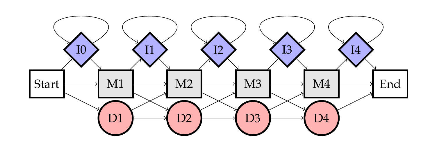
Fig. 13.1 A state diagram of a profile HMM with 4 match states.#
A Profile HMM is structured to mirror the columns of an MSA, with three main states for each column:
Match States (M): Represent conserved positions in the alignment, corresponding to columns with similar residues or nucleotides across multiple sequences. Match states store probabilities for each possible amino acid or nucleotide at that position, reflecting the distribution observed in the MSA.
Insertion States (I): Account for potential insertions between columns, capturing variability by allowing additional residues or nucleotides to be added. These states store probabilities for each possible amino acid or nucleotide to be inserted.
Deletion States (D): Represent positions where sequences may lack a corresponding residue or nucleotide, resulting in a gap in the alignment. Deletion states enable the model to handle varying lengths in sequences.
13.2.3. Emission Probabilities#
Emission probabilities in a Profile HMM quantify the likelihood of observing a specific amino acid or nucleotide at each position in an alignment. These probabilities are stored within match, insertion states (delete states are silent and dont emit sequence) and are derived from the frequencies of residues or nucleotides observed in the Multiple Sequence Alignment (MSA) used to construct the model. Mathematically, the emission probability \(e_i(x)\) for observing residue \(x\) at position \(i\) in the alignment is calculated as:
\(e_i(x) = \frac{{\text{{Count of residue }} x \text{{ at position }} i}}{{\text{{Total count of residues at position }} i}}\).
Here, \(i\) represents the position in the alignment, and \(x\) represents a specific amino acid or nucleotide. The count of residue \(x\) at position \(i\) is divided by the total count of residues at position \(i\) to normalize the probability. Emission probabilities reflect the amino acid composition of each column in the MSA. Unevenly distributed emission probabilities indicate positions that are more conserved, where a specific amino acid or nucleotide is frequently observed across sequences in the alignment. Conversely, evenly distributed emission probabilities suggest positions with more variability, where multiple residues or nucleotides may be present.
13.2.4. Transition Probabilities#
Transition probabilities in a Profile HMM govern the likelihood of transitioning between different states within the model. These probabilities capture the patterns of insertions, deletions, and matches observed in the MSA. Mathematically, the transition probability \(t_{ij}\) from state \(i\) to state \(j\) is calculated as:
\(t_{ij} = \frac{{\text{{Count of transitions from state }} i \text{{ to state }} j}}{{\text{{Total count of transitions from state }} i}}\)
Here, \(i\) and \(j\) represent different states in the model, such as match, insertion, or deletion states. The count of transitions from state \(i\) to state \(j\) is divided by the total count of transitions originating from state \(i\) to normalize the probability. Transition probabilities reflect the probabilities of insertions, deletions, and matches within the MSA. Higher transition probabilities between match states indicate regions of sequence conservation, where consecutive residues are more likely to align without gaps. Conversely, higher transition probabilities from match states to insertion or deletion states suggest regions with more variability, where insertions or deletions are common. By capturing these probabilities, Profile HMMs effectively model the indel patterns observed in the alignment.
13.3. Calculating Sequence Probability Using Profile HMMs#
Before delving into the computational dynamics of the Viterbi algorithm for sequence alignment using Profile Hidden Markov Models (HMMs), we investigate how to calculate the probability of observing a specific sequence along a particular path through the model.
13.3.1. Sequence and Path Definition#
Consider a sequence \(X = x_1, x_2, ..., x_L\) and a corresponding path \(\pi = \pi_1, \pi_2, ..., \pi_L\) through a Profile HMM, where each \(\pi_i\) represents the state (Match, Insertion, or Deletion) at position \(i\) in the sequence. Each state in the path emits a sequence character (deletion states, which are silent, emits a token \(x_i=\delta\) with a probability \(e_{\pi_i}(\delta)=1\)), and the transition from one state to the next is governed by the structure of the HMM.
13.3.2. Probability Calculation#
For Profile HMMs, just as other HMMs, we assume conditional independence of the emitted sequence given its path through the states. This means that the probability of observing a particular sequence is determined solely by the sequence of states in the HMM, independent of the emissions from other states. The probability of observing the sequence \(X\) along the path \(\pi\) through the Profile HMM is then becomming the product of all relevant emission probabilities and transition probabilities along the path. Mathematically, this is expressed as:
\( P(X, \pi) = \prod_{i=1}^{L} e_{\pi_i}(x_i) \cdot t_{\pi_{i}, \pi_{i+1}} \)
Here, \(e_{ \pi_i}(x_i) \) represents the emission probability of observing symbol \(x_i\) from state \(\pi_i\), and \( t_{\pi_{i}, \pi_{i+1}} \) is the transition probability from state \(\pi_i\) to state \(\pi_{i+1}\). It’s important to note that the emission probability of a deletion state is always \(1\) since deletions do not emit any symbols, and hence emits “no symbol” with a probability of \(1\).
13.3.2.1. Step-by-Step Breakdown#
Initialization: Start from the beginning of the sequence and the corresponding initial state in the path. The initial state typically has no preceding state, so the initial transition probability may be a special case, often set based on the model’s parameters.
Iteration: For each position \(i\) from 1 to \(L\) in the sequence and path:
Compute the emission probability \(e_{\pi_i}(x_i)\) if \(\pi_i\) is a match or insertion state. For deletion states, this value is 1.
Compute the transition probability \(t_{\pi_{i-1}, \pi_i}\) from the previous state \(\pi_{i-1}\) to the current state \(\pi_i\).
Multiplication: Multiply all computed probabilities (emission and transition) to get the total probability of observing the sequence \(X\) given the path \(\pi\).
13.4. Sequence Alignment with Profile HMMs using Viterbi Algorithm#
When we want to score a sequence with a profile HMM, we normally don’t have a path available that likely generated a certain sequence. However, it turns out that we can use dynamic programming to find an optimal path. This is done using the Viterbi algorithm, adapted for Profile Hidden Markov Models (Profile HMMs). Here’s a concise breakdown of the process:
13.4.1. Overview:#
Given a Profile HMM and a query sequence, the Viterbi algorithm identifies the most probable alignment between the sequence and the model. This alignment accounts for matches, insertions, and deletions.
13.4.1.1. Steps:#
Initialization:
Initialize the first column of the Viterbi matrix with the emission probabilities for the first residue of the sequence in each match state.
The formula for initialization: \( V(0, 0) = 1.0 \)
Recursion:
Iterate through each residue in the sequence, updating the Viterbi matrix based on transition and emission probabilities.
Update each cell in the Viterbi matrix using the following formula: \( V(i, j) = \max_{k \le j} [V(i-1, k) \cdot t_{kj}] \cdot e_j(x_i), \) when \(j\) is a match or insert state. \( V(i, j) = \max_{k<j} [V(i, k) \cdot t_{kj}], \) when \(j\) is a delete state.
Termination:
Once the entire sequence has been processed, identify the highest probability in the last column of the Viterbi matrix. This represents the likelihood of the most probable path through the model.
Backtracking:
Trace back through the Viterbi matrix, starting from the cell with the highest probability in the last column. Record the path through the model that corresponds to this maximum probability.
Alignment:
Translate the identified path into an alignment between the query sequence and the Profile HMM, where match states represent aligned residues, insertion states represent gaps in the query sequence, and deletion states represent gaps in the model.
13.5. Comparison to MSAs#
13.5.1. Advantages#
Profile HMMs provide a probabilistic framework that captures the variability and evolutionary patterns within multiple sequence alignments (MSAs), allowing for more flexible and robust sequence comparison. Unlike traditional MSAs, Profile HMMs can incorporate gap penalties and position-specific scoring, making them more suitable for handling insertions and deletions. Additionally, Profile HMMs can model the evolutionary history of sequences and predict the likelihood of a sequence being a member of a protein family, which MSAs do not inherently provide.
13.5.2. Disadvantages#
Despite their strengths, Profile HMMs have limitations. The conditional independence criterion, which assumes that the emitted sequence is independent of other emissions given the hidden state, can limit the model’s ability to capture correlations between different positions in the sequence. As a result, Profile HMMs may model interdependencies between positions within a sequence. I.e. if amino acids covary between two positions in a sequence the HMM will not be able to recognize such a pattern.