Multiple Hypothesis Corrections

Introduction¶

In high-throughput biology, analysis often involves testing a large number of hypotheses simultaneously. This is common in fields like genomics, transcriptomics, and proteomics, where experiments might involve thousands of genes or proteins being tested for associations with a condition or trait. When many tests are conducted, even a small chance of error for each test accumulates into a substantial number of false discoveries. Crucially, a single $p$ value can no longer be interpreted in isolation—its meaning depends on the size of the full hypothesis set and on how many results are declared significant.

To understand this, imagine testing 1,000 hypotheses with a significance threshold ($\alpha$) of 0.05. If the null hypothesis is true for all these tests, we would still expect about 5% of them, or 50 tests, to be significant simply by chance. A realistic report therefore needs to communicate both numbers: how many hypotheses were tested and how many were called significant. Only then can we judge whether the significant subset looks plausible or if it is essentially the handful of false positives that we inevitably expect among thousands of null tests.

Multiple hypothesis corrections control an error rate defined over the whole list of significant findings. The two most common ones are the Family-Wise Error Rate (FWER), the probability that the list contains at least one false positive, and the False Discovery Rate (FDR), the expected proportion of false positives in the list.

Bonferroni Correction¶

The Bonferroni correction is one of the simplest and most conservative methods for controlling the FWER. It works as follows:

1. Given a significance level $\alpha$, divide it by the number of hypotheses $m$ being tested to obtain the adjusted significance level:

   $$\alpha_{\text{adjusted}} = \frac{\alpha}{m}$$

   (1)

2. Call a hypothesis significant if its $p$ value is less than $\alpha_{\text{adjusted}}$.

This keeps the probability of making at least one false positive across all the tests below $\alpha$. The price is that with a large number of hypotheses the adjusted threshold becomes so small that many true effects are missed, i.e. the procedure loses statistical power.

Calculating the Upper Bound of the False Discovery Rate with the Benjamini-Hochberg Procedure¶

The Benjamini-Hochberg (BH) procedure is a popular method for controlling the False Discovery Rate (FDR), which is the expected proportion of nulls among the $p$ values below threshold, i.e. the fraction of false positives among the $p$ values we call significant. Unlike the Bonferroni correction, which limits the probability of making even a single false positive, the BH procedure accepts a controlled fraction of false positives in exchange for detecting more of the true effects.

The procedure works as follows:

1. Rank all the $p$ values such that $p_{(1)} \le p_{(2)} \le \dots \le p_{(m)}$, where $m$ is the total number of hypotheses.

2. Choose a desired FDR level, denoted as $q^*$.

3. For each $p$ value $p_{(i)}$, calculate the threshold value

   $$\text{Threshold} = \frac{i}{m} \times q^*$$

   (2)

   where $i$ is the rank of the $p$ value.

4. Find the largest $i$ for which $p_{(i)} \le \frac{i}{m} \times q^*$. Reject the null hypotheses of all tests with $p$ values less than or equal to $p_{(i)}$, i.e. declare those features significant. (If no such $i$ exists, nothing is declared significant.)

The BH procedure guarantees an FDR of at most $q^*$ when the tests are independent, and more generally under positive regression dependence; under arbitrary dependence the threshold has to be divided by $\sum_{k=1}^{m} 1/k \approx \ln m + 0.577$. More precisely, BH controls the FDR at $\pi_0 q^*$ rather than at $q^*$, where $\pi_0$ is the unknown proportion of true null hypotheses, so it is conservative when many of the hypotheses are truly alternative. That is exactly the slack the procedure described next recovers.

Calculating $q$ values with Storey’s Method¶

Storey introduced an alternative to the Benjamini-Hochberg procedure for controlling the FDR, known as the $q$ value approach. The $q$ value is the FDR analogue of the $p$ value: just as the $p$ value of a feature is the smallest significance level at which that feature would be called significant, its $q$ value is the smallest false discovery rate at which it would be called significant, $\hat{q}(p_i) = \min_{t \ge p_i} \hat{\rm FDR}(t)$. Note that this is a minimum over all thresholds at least as large as $p_i$, and not simply the estimated FDR evaluated at $p_i$; since $\hat{\rm FDR}(t)$ is not monotone in $t$, the two can differ.

Both Storey’s method and the Benjamini-Hochberg procedure view the observed $p$ values as a mixture of two groups: $p$ values from true null hypotheses ($H_0$), which are uniformly distributed between 0 and 1, and $p$ values from true alternative hypotheses ($H_1$), which tend to be small. The Benjamini-Hochberg procedure in effect assumes that all hypotheses are null when it counts the expected false positives, while Storey’s method estimates the fraction $\pi_0$ of the $p$ values that stem from true null hypotheses.

Storey’s procedure counts the features considered significant as the $p$ values below a threshold $t$. The number of nulls below this threshold is estimated as $\pi_0 m t$, where $\pi_0$ is the estimated fraction of null hypotheses, $m$ is the total number of hypotheses, and $t$ is the chosen threshold. This is possible because we expect $\pi_0 m$ nulls, uniformly distributed between 0 and 1, and a fraction $t$ of them to fall below the threshold.

The proportion of null statistics $\pi_0$ is estimated by a procedure of its own. If all hypotheses were null, we would expect approximately $m(1 - \lambda)$ $p$ values above a threshold $\lambda$. Alternative $p$ values rarely end up above $\lambda$, so the number of $p$ values above $\lambda$, divided by $m(1 - \lambda)$, estimates $\pi_0$. As $\lambda$ approaches 1, this estimate contains fewer alternative $p$ values but the estimate also becomes more variable, so a smoothing function (spline) is applied to stabilize the estimate by evaluating it at $\lambda = 1$.

Here is how Storey’s $q$ value procedure works, as described by Storey & Tibshirani:

1. Order the $p$ values: Let $p_{(1)} \le p_{(2)} \le \dots \le p_{(m)}$ be the ordered $p$ values. Lower $p$ values indicate stronger evidence against the null hypothesis.

2. Estimate $\pi_0$ for a range of $\lambda$ values:

   • For a range of $\lambda$ values, such as $\lambda = 0, 0.05, 0.10, \dots, 0.95$, calculate the proportion of $p$ values greater than $\lambda$:

   $$\hat{\pi}_0(\lambda) = \frac{|\{ p_i > \lambda \}|}{m (1 - \lambda)}$$

   (3)

   where $|\{ p_i > \lambda \}|$ represents the count of $p$ values greater than $\lambda$, and $m$ is the total number of hypotheses.

3. Fit a natural cubic spline to estimate $\pi_0$:

   • Let $\hat{f}$ be a natural cubic spline with three degrees of freedom, fitted to $\hat{\pi}_0(\lambda)$ as a function of $\lambda$. The final estimate of $\pi_0$ is given by evaluating the spline at $\lambda = 1$:

   $$\hat{\pi}_0 = \hat{f}(1)$$

   (4)

   A spline is a smooth curve made of polynomial pieces. With only three degrees of freedom the spline does not pass through every $\hat{\pi}_0(\lambda)$; it smooths out their random fluctuations, which are largest for $\lambda$ close to 1.

4. Estimate the FDR for each $p$ value:

   • Estimate the FDR for a threshold $t=p_{(i)}$ at each ordered $p$ value, as the estimated number of significant null statistics, $\hat{\pi}_0 m p_{(i)}$, divided by the number of $p$ values below or at the threshold, $i$.

   $$\hat{\rm FDR}(t=p_{(i)}) = \frac{\hat{\pi}_0 m p_{(i)}}{i}$$

   (5)

5. Ensure monotonicity:

   • Assign $\hat{q}_{(m)} = \hat{\rm FDR}(t=p_{(m)}) = \hat{\pi}_0 p_{(m)}$

   • For $i = m - 1, m - 2, \dots, 1$, update the $q$ values to ensure they are monotonically increasing:

   $$\hat{q}_{(i)} = \min(\hat{\rm FDR}(t=p_{(i)}), \hat{q}_{(i+1)})$$

   (6)

   This way a larger $p$ value never receives a smaller $q$ value.

If we set $\hat{\pi}_0=1$, Storey’s procedure calls exactly the same features significant at an FDR level $q^*$ as the Benjamini-Hochberg procedure. As long as $\hat{\pi}_0 \le 1$, Storey’s method is therefore never more conservative than Benjamini-Hochberg, and it gains the most power when many hypotheses are truly alternative, i.e. when $\pi_0$ is well below one.

Illustration: true and false positives in a $p$ value histogram¶

Below we simulate $p$ values for 1,000 hypotheses, half of which are nulls (no effect) and half alternative hypotheses (a true effect).

# When the page runs in the browser (JupyterLite), seaborn is not preinstalled, so we install it first
import sys
if sys.platform == "emscripten":
    import micropip
    await micropip.install("seaborn")

Source

import numpy as np
import seaborn as sns
import matplotlib.pyplot as plt

# Parameters
rng = np.random.default_rng(42)
m = 1000  # Number of hypotheses
true_null_proportion = 0.5  # Proportion of null hypotheses

true_nulls = int(m * true_null_proportion)
alternative = m - true_nulls

# Generate p-values from uniform distribution for nulls
p_values_null = rng.uniform(0, 1, true_nulls)

# Generate p-values from a Beta distribution for false nulls (to represent true effects)
p_values_effect = rng.beta(1.0, 5.0, alternative)  # Just for illustration

# Combine p-values
p_values = np.concatenate([p_values_null, p_values_effect])

# Plot the p value distribution
sns.set(style="whitegrid", context="talk")
plt.figure(figsize=(14, 6))
sns.histplot(p_values, bins=50, kde=False, color='gray', alpha=0.5, label='$p$ values')
plt.axvline(x=0.1, color='r', linestyle='--', label='Significance Threshold')
plt.axhline(y=true_nulls / 50, color='b', linestyle='--', label='Expected Level of Nulls')

# Add text for TP, FP, FN, TN
plt.text(0.05, plt.ylim()[1] * 0.2, 'TP', color='green', fontsize=20, horizontalalignment='center')
plt.text(0.05, plt.ylim()[1] * 0.05, 'FP', color='red', fontsize=20, horizontalalignment='center')
plt.text(0.15, plt.ylim()[1] * 0.2, 'FN', color='blue', fontsize=20, horizontalalignment='center')
plt.text(0.15, plt.ylim()[1] * 0.05, 'TN', color='purple', fontsize=20, horizontalalignment='center')

plt.xlabel('$p$ value')
plt.ylabel('Frequency')
plt.xlim(0., 1.)
plt.legend()
plt.show()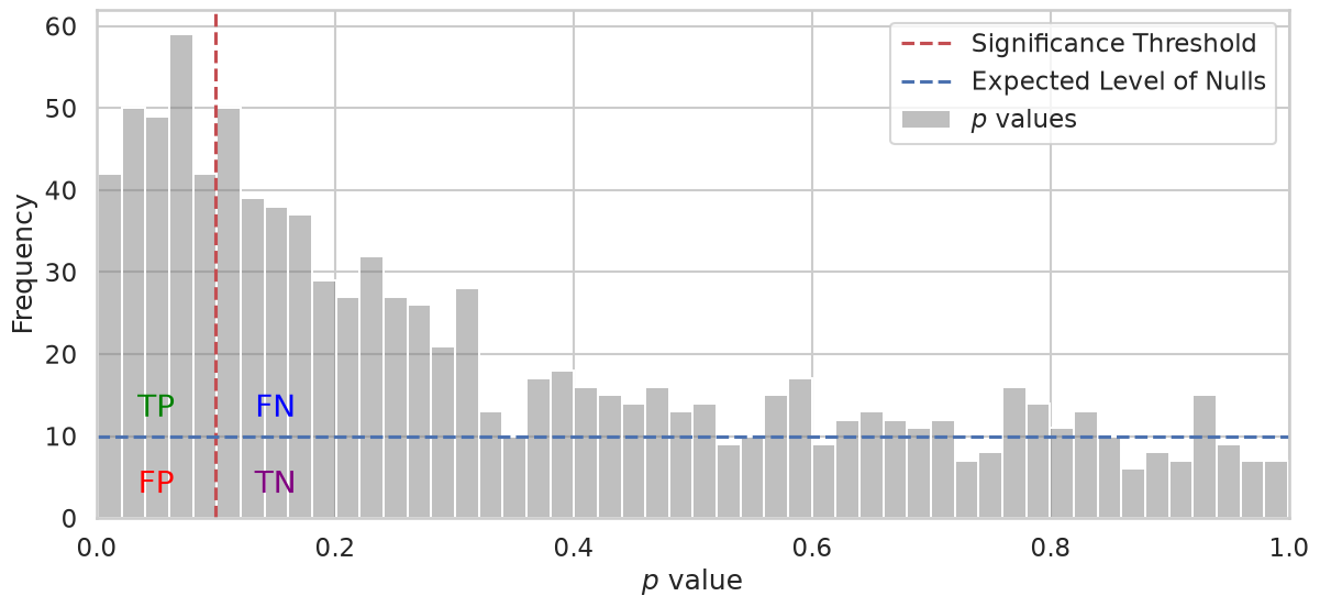

The $p$ values of the nulls are uniformly distributed between 0 and 1, which gives the flat part of the histogram. This follows from the way a $p$ value is constructed: if the test statistic $T$ has a continuous cumulative distribution $F$ under the null, then $p = 1 - F(T)$, and applying a distribution function to its own random variable always yields a uniform variable, so $\Pr(p \le u) = u$ for every $u$ in $[0,1]$ whatever the shape of $F$. The $p$ values of the alternative hypotheses are concentrated near zero, as data generated with a true effect are unlikely under the null hypothesis.

True and false positives¶

The vertical red line marks a significance threshold: hypotheses with $p$ values at or below it are called significant, those above it not significant. The dashed blue line marks the expected height of the histogram for the null $p$ values alone. Together, the two lines divide the hypotheses into four groups:

• TP (True Positives): alternative hypotheses below the threshold, i.e. real effects that we correctly identify.

• FP (False Positives): null hypotheses that end up below the threshold due to random variation.

• FN (False Negatives): alternative hypotheses above the threshold, i.e. true effects that we fail to detect. A high number of FNs means that our test lacks sensitivity.

• TN (True Negatives): null hypotheses above the threshold.

The FDR, the expected proportion of false positives among all hypotheses called significant, is then approximately

Moving the threshold trades sensitivity, the fraction of the true effects that we detect, against precision, $1-\text{FDR}$, the fraction of our findings that are real.