Clustering

Introduction¶

Unsupervised machine learning learns patterns from data without predefined labels. Formally, the goal is to learn a function $f(\mathbf{x})$ from the dataset $D = \{\mathbf{x}_i\}$ by optimizing an objective function $g(D, f)$, or simply to partition $D$. The PCA chapter learned such a function, the projection onto the directions of largest variation. This chapter turns to clustering, which partitions the data into groups such that the data points within a group are similar to each other.

Clustering methods can be divided into hard clustering, in which each data point is assigned to exactly one cluster, and soft (fuzzy) clustering, in which a data point can belong to several clusters with different probabilities.

k-means clustering¶

One of the most common clustering algorithms is k-means, a hard clustering algorithm. It partitions the data points $\mathbf{x}_p$ into $k$ clusters $S_1, \ldots, S_k$ with centers $\mathbf{m}_1, \ldots, \mathbf{m}_k$, so that the within-cluster sum of squared Euclidean distances, also called the inertia,

is as small as possible.

Algorithm overview¶

Starting from $k$ initial centers, k-means alternates between two steps:

• Cluster assignment: Each data point is assigned to the nearest cluster center:

  $$S_i^{(t)} = \{\mathbf{x}_p: \lVert\mathbf{x}_p - \mathbf{m}_i^{(t)}\rVert^2 \le \lVert\mathbf{x}_p - \mathbf{m}_j^{(t)}\rVert^2 \; \forall j \}$$

  (2)

• Recalculation of cluster centers: Each center is recalculated as the arithmetic mean of the data points assigned to it:

  $$\mathbf{m}_i^{(t+1)} = \frac{1}{|S_i^{(t)}|} \sum_{\mathbf{x}_p \in S_i^{(t)}} \mathbf{x}_p$$

  (3)

These steps are repeated until the cluster assignments no longer change. Neither step can increase $J$, so the algorithm always converges, but only to a local minimum of $J$ that depends on the initial centers.

Illustrations of k-means¶

The figure below follows k-means through its first three iterations. The assignment steps are labelled E-steps and the recalculation steps M-steps, names that will make sense when we meet the EM algorithm below.

# When the page runs in the browser (JupyterLite), seaborn is not preinstalled, so we install it first
import sys
if sys.platform == "emscripten":
    import micropip
    await micropip.install("seaborn")

import numpy as np
from sklearn.metrics import pairwise_distances_argmin
from sklearn.datasets import make_blobs
import seaborn as sns
import matplotlib.pyplot as plt

# Generate sample data
X, y_true = make_blobs(n_samples=300, centers=5, cluster_std=0.60, random_state=1)

# Function to plot data points with cluster centers
def plot_kmeans_step(ax, X, centers, labels=None, step_title=""):
    if labels is not None:
        ax.scatter(X[:, 0], X[:, 1], c=labels, s=50, cmap='plasma', label='Data Points')
    else:
        ax.scatter(X[:, 0], X[:, 1], color='gray', s=50, alpha=0.6, label='Data Points')
    sns.scatterplot(x=centers[:, 0], y=centers[:, 1], color='black', s=200, alpha=0.5, ax=ax, label='Cluster Centers')
    ax.set_title(step_title)

# Initialize the plot with a 4x2 grid (from the second row on, E-steps on the left and M-steps on the right)
fig, axes = plt.subplots(4, 2, figsize=(12, 16))
fig.tight_layout(pad=5)

# Step 0: The data before clustering
axes[0, 0].scatter(X[:, 0], X[:, 1], color='gray', s=50, alpha=0.6)
axes[0, 0].set_title("Data Points")

# Step 1: Initial Random Cluster Centers
rng = np.random.RandomState(1)
i = rng.permutation(X.shape[0])[:5]
centers = X[i]
plot_kmeans_step(axes[0, 1], X, centers, step_title="Initial Random Cluster Centers")

# Step 2: First E-Step (assign points to the nearest cluster center)
labels = pairwise_distances_argmin(X, centers)
plot_kmeans_step(axes[1, 0], X, centers, labels, "First E-Step: Assign Points to Nearest Cluster")

# Step 3: First M-Step (recalculate cluster centers)
centers = np.array([X[labels == i].mean(axis=0) for i in range(len(centers))])
plot_kmeans_step(axes[1, 1], X, centers, labels, step_title="First M-Step: Recalculate Cluster Centers")

# Step 4: Second E-Step (assign points to the nearest cluster center)
labels = pairwise_distances_argmin(X, centers)
plot_kmeans_step(axes[2, 0], X, centers, labels, "Second E-Step: Assign Points to Nearest Cluster")

# Step 5: Second M-Step (recalculate cluster centers)
centers = np.array([X[labels == i].mean(axis=0) for i in range(len(centers))])
plot_kmeans_step(axes[2, 1], X, centers, labels, step_title="Second M-Step: Recalculate Cluster Centers")

# Step 6: Third E-Step (assign points to the nearest cluster center)
labels = pairwise_distances_argmin(X, centers)
plot_kmeans_step(axes[3, 0], X, centers, labels, "Third E-Step: Assign Points to Nearest Cluster")

# Step 7: Third M-Step (recalculate cluster centers)
centers = np.array([X[labels == i].mean(axis=0) for i in range(len(centers))])
plot_kmeans_step(axes[3, 1], X, centers, labels, step_title="Third M-Step: Recalculate Cluster Centers")

plt.show()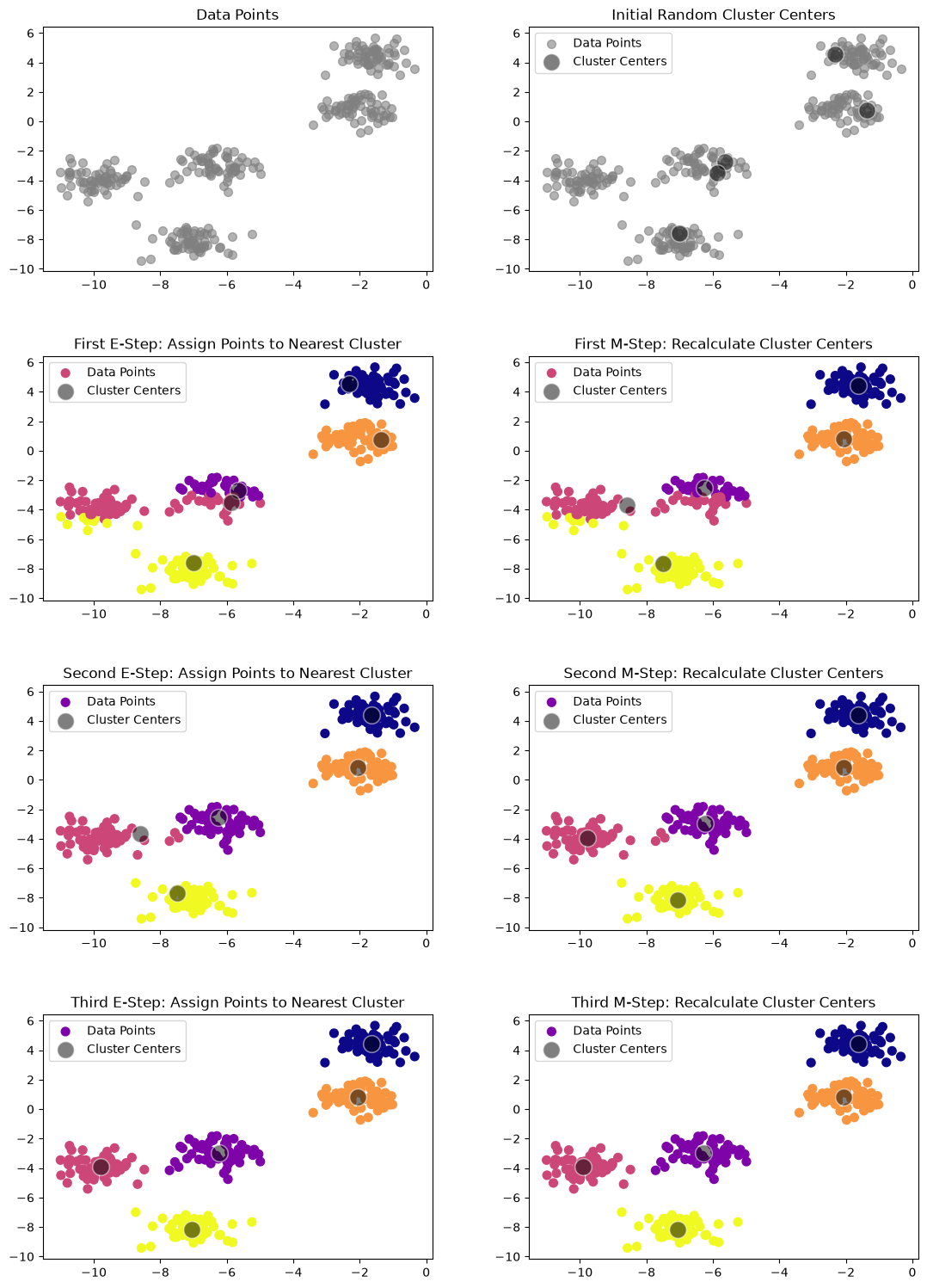

The algorithm automatically assigns the points to clusters, and we can see that it closely matches what we would expect by visual inspection.

Voronoi cells and k-means clustering¶

The k-means clusters form Voronoi cells: each point in the cell of a cluster center is closer to that center than to any other center. The border between two neighbouring cells consists of the points at equal distance from both centers, which is a straight line (in more dimensions, a plane), so k-means always separates its clusters by linear boundaries. The script below draws the Voronoi cells of 7 randomly positioned cluster centers in two dimensions.

import numpy as np
import matplotlib.pyplot as plt
from scipy.spatial import Voronoi, voronoi_plot_2d

# Generate 7 random cluster centers in 2D space
np.random.seed(0)  # For reproducibility
cluster_centers = np.random.rand(7, 2) * 10

# Compute Voronoi diagram
vor = Voronoi(cluster_centers)

# Plot Voronoi diagram
fig, ax = plt.subplots()
voronoi_plot_2d(vor, ax=ax, show_vertices=False, line_colors='orange', line_width=2, line_alpha=0.6, point_size=10)

# Plot cluster centers
ax.plot(cluster_centers[:, 0], cluster_centers[:, 1], 'bo', markersize=8, label='Cluster Centers')

# Add labels and title
ax.set_title('Voronoi Cells of 7 Random Cluster Centers')
ax.set_xlabel('X-axis')
ax.set_ylabel('Y-axis')
ax.legend()
plt.xlim(0, 10)
plt.ylim(0, 10)
plt.grid()
plt.show()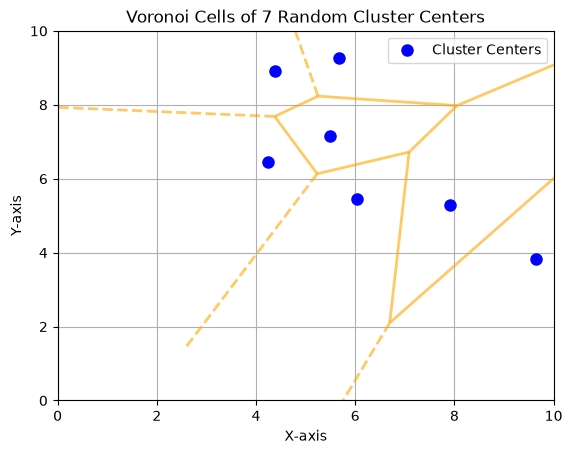

Drawbacks of k-means¶

The k-means algorithm is simple and effective, but it has some drawbacks:

1. Initialization sensitivity: The algorithm’s result can be highly dependent on the initial choice of cluster centers. Poor initialization may lead to suboptimal clustering, as k-means may converge to a local minimum of $J$. For example, using a different random seed can lead to different cluster assignments.

2. Predefined number of clusters: k-means requires specifying the number of clusters beforehand. For example, if we set the number of clusters to three instead of five, the algorithm will still proceed, but the result may not be meaningful.

from sklearn.cluster import KMeans

labels = KMeans(3, random_state=0).fit_predict(X)
plt.scatter(X[:, 0], X[:, 1], c=labels, s=50, cmap='plasma');
plt.show()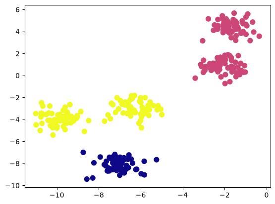

3. Linear cluster boundaries: The k-means algorithm assumes that clusters are spherical and separated by linear boundaries. It struggles with complex geometries. Consider the following dataset with two crescent-shaped clusters:

from sklearn.datasets import make_moons

X, y = make_moons(200, noise=.05, random_state=42)
labels = KMeans(2, random_state=0).fit_predict(X)
plt.scatter(X[:, 0], X[:, 1], c=labels, s=50, cmap='plasma');
plt.show()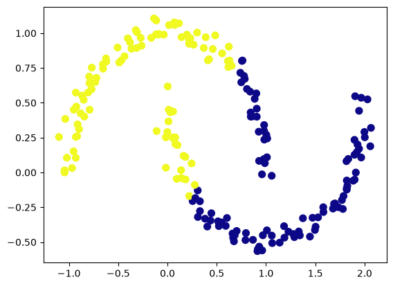

4. Differences in Euclidean size: k-means assumes that all clusters have fairly similar sizes, in terms of the Euclidean distance from their center to their border. Here is an example of three clusters arranged like the head and ears of Mickey Mouse, where k-means has a hard time placing the cluster borders correctly.

from matplotlib.lines import Line2D

# Parameters for the blobs
n_samples = [600, 100, 100]  
centers = [(0, 0), (3, 3), (-3, 3)]  # Center coordinates
cluster_std = [2., 0.5, 0.5]  # Standard deviations for each blob

# Generate blobs
X, y = make_blobs(n_samples=n_samples, centers=centers, cluster_std=cluster_std, random_state=1)

labels = KMeans(3, random_state=0).fit_predict(X)
# The marker shape shows the blob a point was generated from (circle, square, diamond),
# the colour shows the k-means cluster it was assigned to
markers = ['o', 's', 'D']

plt.figure(figsize=(8, 6))
for i in range(3):
    plt.scatter(X[y == i, 0], X[y == i, 1], c=labels[y == i], cmap='plasma', vmin=0, vmax=2,
                marker=markers[i], edgecolor='k', s=50)
# The legend explains the marker shapes, so its symbols are drawn in gray
shape_legend = [Line2D([], [], marker=m, linestyle='', markerfacecolor='lightgray',
                       markeredgecolor='k', markersize=8, label=f"Blob {i+1}")
                for i, m in enumerate(markers)]
plt.legend(handles=shape_legend, title="Generated from", loc='upper right')
plt.title("Generated blobs (marker shape) and k-means clusters (colour)")
plt.xlabel("Feature 1")
plt.ylabel("Feature 2")
plt.grid(True)
plt.show()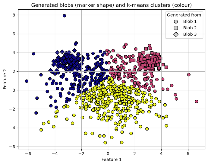

Multivariate normal distribution¶

A multivariate normal distribution, also known as a multinormal distribution, is a generalization of the one-dimensional normal distribution to multiple dimensions.

Definition¶

A multivariate normal distribution is characterized by a vector of mean values ($\boldsymbol{\mu}$) and a covariance matrix ($\boldsymbol{\Sigma}$). It describes the joint distribution of a set of random variables, each of which has a univariate normal distribution, but with the potential for covariance between them, allowing for dependencies. Mathematically, if $\mathbf{X}$ is a random vector $(X_1, X_2, \dots, X_d)$ following a multivariate normal distribution, its probability density function is given by:

where:

• $\mathbf{x}$ is a real $d$-dimensional vector,

• $\boldsymbol{\mu}$ is the mean vector,

• $\boldsymbol{\Sigma}$ is the $d \times d$ covariance matrix,

• $d$ is the number of dimensions (variables),

• $|\boldsymbol{\Sigma}|$ is the determinant of the covariance matrix.

The multivariate normal distribution is the building block of the Gaussian mixture models below.

Source

import numpy as np
import matplotlib.pyplot as plt
from scipy.stats import multivariate_normal

# Parameters for the bivariate normal distribution
mean = [0, 0]  # Mean vector
cov = [[1, 0.5], [0.5, 1]]  # Covariance matrix

# Generate grid points for plotting
x = np.linspace(-3, 3, 100)
y = np.linspace(-3, 3, 100)
X, Y = np.meshgrid(x, y)
pos = np.dstack((X, Y))

# Calculate the probability density function
rv = multivariate_normal(mean, cov)
Z = rv.pdf(pos)

# Create a figure with two subplots: a 3D surface and a 2D contour plot
fig = plt.figure(figsize=(12, 6))

# 3D Surface plot
ax = fig.add_subplot(1, 2, 1, projection='3d')
ax.plot_surface(X, Y, Z, cmap='viridis', edgecolor='k', alpha=0.7)
ax.set_title("3D Surface Plot of Bivariate Normal Distribution")
ax.set_xlabel("X-axis")
ax.set_ylabel("Y-axis")
ax.set_zlabel("Density")

# 2D Contour plot
ax2 = fig.add_subplot(1, 2, 2)
contour = ax2.contourf(X, Y, Z, cmap='viridis')
plt.colorbar(contour, ax=ax2, label="Density")
ax2.set_title("2D Contour Plot of Bivariate Normal Distribution")
ax2.set_xlabel("X-axis")
ax2.set_ylabel("Y-axis")

plt.tight_layout()
plt.show()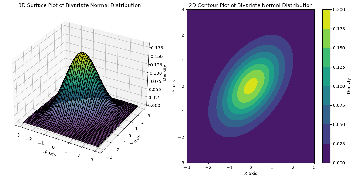

Gaussian mixture models (GMM)¶

Gaussian mixture models (GMMs) are a probabilistic, soft clustering method. They assume that the data were generated from a mixture of several multivariate normal distributions, one for each cluster, which makes them flexible enough to model clusters of different sizes, shapes and orientations.

Mathematical formulation¶

We model the data as generated from a mixture of $K$ components. Component $k$ is a multivariate normal distribution $\mathcal{N}(\mathbf{x}|\boldsymbol{\mu}_k, \boldsymbol{\Sigma}_k)$ with its own mean $\boldsymbol{\mu}_k$ and covariance matrix $\boldsymbol{\Sigma}_k$, and it has a mixing coefficient $P_k$, the proportion of data points that belong to it. The probability density function of a GMM with $K$ components is

The EM algorithm¶

The parameters of a GMM are fitted with the expectation-maximization (EM) algorithm, a general method for fitting models in which some information is hidden. Such unobserved quantities are called latent variables. In a GMM, the latent variable is the cluster membership of each data point: we never observe which component generated a point. The means, covariance matrices and mixing coefficients, in contrast, are model parameters. EM alternates between estimating the memberships from the current parameters (E-step) and re-estimating the parameters from the memberships (M-step):

1. Initialization: Choose the number of components $K$ and initial values for the means $\boldsymbol{\mu}_k$, the covariance matrices $\boldsymbol{\Sigma}_k$ and the mixing coefficients $P_k$, with $\sum_{k=1}^K P_k = 1$.

2. Expectation step (E-step): Compute the probability that data point $\mathbf{x}_n$ was generated by component $k$, called the responsibility $\gamma_{nk}$:

   $$\gamma_{nk} = \frac{P_k \mathcal{N}(\mathbf{x}_n | \boldsymbol{\mu}_k, \boldsymbol{\Sigma}_k)}{\sum_{j=1}^K P_j \mathcal{N}(\mathbf{x}_n | \boldsymbol{\mu}_j, \boldsymbol{\Sigma}_j)}$$

   (6)

   where $\mathcal{N}(\mathbf{x}_n | \boldsymbol{\mu}_k, \boldsymbol{\Sigma}_k)$ is the multivariate normal density defined above.

3. Maximization step (M-step): Re-estimate the parameters from the responsibilities, choosing the values that maximize the likelihood of the data given these soft assignments. With $N_k = \sum_{n=1}^N \gamma_{nk}$, the effective number of points in component $k$, the updates are

   $$\boldsymbol{\mu}_k^{\text{new}} = \frac{1}{N_k} \sum_{n=1}^N \gamma_{nk} \mathbf{x}_n$$

   (7)
   $$\boldsymbol{\Sigma}_k^{\text{new}} = \frac{1}{N_k} \sum_{n=1}^N \gamma_{nk} (\mathbf{x}_n - \boldsymbol{\mu}_k^{\text{new}})(\mathbf{x}_n - \boldsymbol{\mu}_k^{\text{new}})^{\textsf{T}}$$

   (8)
   $$P_k^{\text{new}} = \frac{N_k}{N}$$

   (9)

4. Convergence check: Evaluate the log-likelihood of the data given the current parameters,

   $$\ln \Pr(\mathbf{X} | \boldsymbol{\mu}, \boldsymbol{\Sigma}, \mathbf{P}) = \sum_{n=1}^N \ln \left( \sum_{k=1}^K P_k \mathcal{N}(\mathbf{x}_n | \boldsymbol{\mu}_k, \boldsymbol{\Sigma}_k) \right)$$

   (10)

   and repeat steps 2 and 3 until it no longer increases.

k-means can be seen as a special case of EM in which cluster membership is a hard 0 or 1 assignment instead of a probability. Its assignment step is an E-step that gives each point responsibility 1 for its nearest center and 0 for all others, and its update step is an M-step that only re-estimates the centers, so as to minimize $J$. A GMM instead keeps soft memberships, so that points near a boundary can belong partly to several clusters, and it also estimates a covariance matrix for each component, so that clusters can be elliptical and oriented in any direction. EM is used well beyond clustering, for instance to fit hidden Markov models, whose latent variables are the hidden states behind an observed sequence, as well as factor analysis and topic models.

Illustrations of GMM¶

1. Correlated features: Here is a set of random data points generated from four normal distributions with correlated features, which gives tilted elliptical clusters.

import numpy as np
import matplotlib.pyplot as plt
from sklearn.mixture import GaussianMixture
from matplotlib.patches import Ellipse

# Function to generate tilted elliptical blobs with custom shapes
def generate_tilted_blobs(means, covariances, n_samples):
    X = []
    y = []
    for i, (mean, cov) in enumerate(zip(means, covariances)):
        # Generate points for each cluster with given mean and covariance
        cluster_points = np.random.multivariate_normal(mean, cov, n_samples)
        X.append(cluster_points)
        y.extend([i] * n_samples)
    X = np.vstack(X)
    y = np.array(y)
    return X, y

# Define means and covariances for tilted elliptical clusters
means = [[0, 0], [-3, 3], [0, 5], [2, 2]]
covariances = [
    [[1, 0.5], [0.5, 1]],  # Slightly rotated ellipse
    [[0.3, 0.2], [0.2, 1.2]],  # Narrow ellipse
    [[1.5, -0.7], [-0.7, 0.5]],  # Wider, tilted ellipse
    [[0.5, -0.3], [-0.3, 0.5]],  # Smaller ellipse
]

# Generate the tilted blobs
np.random.seed(0)  # For reproducibility
X, y_true = generate_tilted_blobs(means, covariances, 100)
plt.scatter(X[:, 0], X[:, 1], s=40)
plt.title("Generated data with tilted elliptical clusters")
plt.show()

# Function to draw ellipses based on covariance matrices
def draw_ellipse(position, covariance, ax=None, **kwargs):
    ax = ax or plt.gca()
    if covariance.shape == (2, 2):
        U, s, Vt = np.linalg.svd(covariance)
        angle = np.degrees(np.arctan2(U[1, 0], U[0, 0]))
        width, height = 2 * np.sqrt(s)
    else:
        angle = 0
        width, height = 2 * np.sqrt(covariance)
    for nsig in range(1, 4):
        ax.add_patch(Ellipse(position, nsig * width, nsig * height, angle=angle, **kwargs))

# Plot GMM with elliptical boundaries
def plot_gmm(gmm, X, label=True, ax=None):
    ax = ax or plt.gca()
    labels = gmm.fit(X).predict(X)
    if label:
        ax.scatter(X[:, 0], X[:, 1], c=labels, s=40, cmap='plasma', zorder=2)
    else:
        ax.scatter(X[:, 0], X[:, 1], s=40, zorder=2)
    ax.axis('equal')
    w_factor = 0.2 / gmm.weights_.max()
    for pos, covar, w in zip(gmm.means_, gmm.covariances_, gmm.weights_):
        draw_ellipse(pos, covar, alpha=w * w_factor)

# Apply Gaussian Mixture Model to generated data
gmm = GaussianMixture(n_components=4, covariance_type='full', random_state=42)
plot_gmm(gmm, X)
plt.title("GMM fitted to tilted elliptical clusters")
plt.show()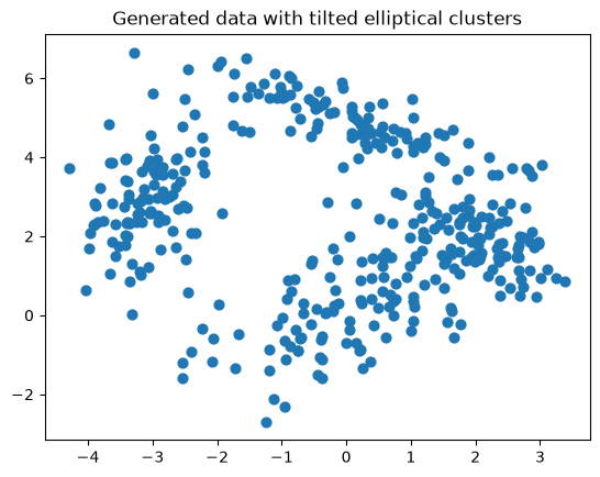

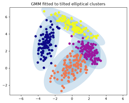
Each fitted component is drawn as ellipses at one, two and three standard deviations, with an opacity proportional to its mixing coefficient, and each point is coloured by the component with the largest responsibility. The fitted components recover the four generated clusters, including their tilts.

2. Clusters of different sizes: Here is a GMM fitted to the same three blobs that k-means split incorrectly above.

# The same blobs as in the k-means example above
n_samples = [600, 100, 100]
centers = [(0, 0), (3, 3), (-3, 3)]  # Center coordinates
cluster_std = [2., 0.5, 0.5]  # Standard deviations for each blob

# Generate blobs
X, y = make_blobs(n_samples=n_samples, centers=centers, cluster_std=cluster_std, random_state=1)

# Plot GMM with elliptical boundaries
gmm = GaussianMixture(n_components=3, covariance_type='full', random_state=42)
plot_gmm(gmm, X)
plt.show()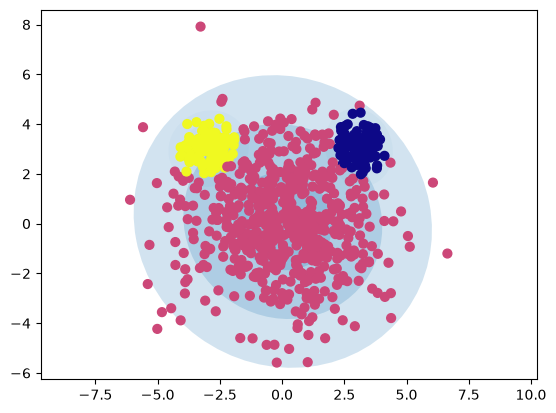

Unlike k-means, the GMM recovers the large, wide blob and the two small ones. It still describes each cluster as a single elliptical blob, however, so it would not cleanly separate the two moons above either.

Comparison between k-means and GMM¶

The following table highlights the similarities and differences between the k-means and GMM algorithms in terms of their iteration steps: