Cluster analysis of single cells

Introduction¶

Clustering single cells is one of the applications that made unsupervised learning a routine tool in molecular biology. A single-cell experiment delivers a matrix of a few thousand cells that were deliberately not labelled — the whole point of the technique is that we do not have to sort the cells beforehand. Recovering the cell types from the expression data alone is exactly the partitioning problem set up in the clustering chapter, and we solve it here with the two algorithms introduced there, k-means and Gaussian mixture models.

We use the same dataset as in the chapter PCA of single cells: the pbmc3k set of roughly 2,700 peripheral blood mononuclear cells from a healthy donor, distributed by 10x Genomics. What makes it valuable for teaching is that we have an independent way of checking the answer. Immunologists have spent decades establishing marker genes that identify blood cell types, so once the algorithm has produced a partition we can ask what each cluster expresses, and judge whether the clusters are real.

The notebook is self-contained, so the loading and preprocessing steps of the single-cell PCA chapter are repeated here without further comment; see that chapter for the reasoning behind each step.

Loading and preprocessing the data¶

# When the page runs in the browser (JupyterLite), we install seaborn, and fetch the data from a copy in the book's
# repository, as the 10x Genomics server does not allow downloads from within a browser
import sys
if sys.platform == "emscripten":
    import os
    import micropip
    await micropip.install(["seaborn", "pyodide-http"])
    import pyodide_http
    pyodide_http.patch_all()
    from urllib.request import urlretrieve
    archive = "../data/pbmc3k_filtered_gene_bc_matrices.tar.gz"
    os.makedirs("../data", exist_ok=True)
    if not os.path.exists(archive):
        urlretrieve("https://raw.githubusercontent.com/statisticalbiotechnology/dsbook/main/dsbook/unsupervised/data/"
                    "pbmc3k_filtered_gene_bc_matrices.tar.gz", archive)
    # scipy's Matrix Market reader starts several threads, which the browser does not support
    import scipy.io._fast_matrix_market
    scipy.io._fast_matrix_market.PARALLELISM = 1

import os
import sys
import tarfile
import requests
import numpy as np
import pandas as pd
import matplotlib.pyplot as plt
import seaborn as sns
from scipy.io import mmread

IN_COLAB = 'google.colab' in sys.modules
data_dir = "data/" if IN_COLAB else "../data/"
os.makedirs(data_dir, exist_ok=True)

url = "https://cf.10xgenomics.com/samples/cell-exp/1.1.0/pbmc3k/pbmc3k_filtered_gene_bc_matrices.tar.gz"
archive = os.path.join(data_dir, "pbmc3k_filtered_gene_bc_matrices.tar.gz")
matrix_dir = os.path.join(data_dir, "filtered_gene_bc_matrices", "hg19")

if not os.path.exists(matrix_dir):
    if not os.path.exists(archive):
        print("Downloading pbmc3k ...")
        response = requests.get(url, stream=True)
        response.raise_for_status()
        with open(archive, "wb") as handle:
            for chunk in response.iter_content(chunk_size=1 << 16):
                handle.write(chunk)
    with tarfile.open(archive, "r:gz") as tar:
        tar.extractall(path=data_dir, filter="data")

counts = mmread(os.path.join(matrix_dir, "matrix.mtx")).T.tocsr()   # cells x genes
genes = pd.read_csv(os.path.join(matrix_dir, "genes.tsv"), sep="\t",
                    header=None, names=["ensembl", "symbol"])
gene_names = genes["symbol"].to_numpy(dtype=str)

Quality control: keep cells with 200–2,500 detected genes and less than 5% mitochondrial counts, and keep genes seen in at least three cells.

total_counts = np.asarray(counts.sum(axis=1)).ravel()
n_genes = np.asarray((counts > 0).sum(axis=1)).ravel()
is_mito = np.char.startswith(gene_names, "MT-")
mito_fraction = np.asarray(counts[:, is_mito].sum(axis=1)).ravel() / total_counts

keep_cells = (n_genes > 200) & (n_genes < 2500) & (mito_fraction < 0.05)
counts = counts[keep_cells]
total_counts = total_counts[keep_cells]

keep_genes = np.asarray((counts > 0).sum(axis=0)).ravel() >= 3
counts = counts[:, keep_genes]
gene_names = gene_names[keep_genes]
print(f"{counts.shape[0]} cells x {counts.shape[1]} genes")

2638 cells x 13656 genes

Normalisation to counts per ten thousand, $\log(1+x)$ transformation, selection of the 1,000 most variable genes, and standardisation.

expression = counts.multiply(1e4 / total_counts[:, None]).tocsr().log1p()
expression = np.asarray(expression.todense())
expression_df = pd.DataFrame(expression, columns=gene_names)

hvg_index = np.argsort(expression.var(axis=0))[::-1][:1000]
X = expression[:, hvg_index]
X = np.clip((X - X.mean(axis=0)) / X.std(axis=0), -10, 10)

Clustering in principal component space¶

As argued at the end of the single-cell PCA chapter, we do not cluster the 1,000-dimensional standardised matrix directly. Both k-means and Gaussian mixture models rely on distances between cells (Euclidean distances for k-means, distances scaled by each component’s variances for a mixture model), and in 1,000 dimensions those distances are dominated by counting noise. We therefore project the cells onto their first 15 principal components and cluster in that subspace.

from sklearn.decomposition import PCA

pca = PCA(n_components=50, random_state=0)
scores = pca.fit_transform(X)
Y = scores[:, :15]          # the space in which we cluster
print("Clustering space:", Y.shape)

Clustering space: (2638, 15)

Choosing the number of clusters¶

k-means requires us to fix the number of clusters $k$ in advance — one of the drawbacks listed in the theory chapter. Two standard diagnostics help us choose. The inertia, that is the within-cluster sum of squared distances $\sum_i \sum_{\mathbf{x} \in S_i} \lVert \mathbf{x}-\mathbf{m}_i \rVert^2$ that k-means minimises, always decreases as $k$ grows, so we look for an elbow where the improvement levels off. The silhouette score compares, for each point, its mean distance to the other members of its own cluster with its mean distance to the members of the nearest other cluster; it is largest when clusters are compact and well separated.

from sklearn.cluster import KMeans
from sklearn.metrics import silhouette_score

ks = range(2, 11)
inertia, silhouette = [], []
for k in ks:
    km = KMeans(n_clusters=k, n_init=10, random_state=0).fit(Y)
    inertia.append(km.inertia_)
    silhouette.append(silhouette_score(Y, km.labels_))

fig, axes = plt.subplots(1, 2, figsize=(11, 4))
axes[0].plot(list(ks), inertia, "o-")
axes[0].set(xlabel="Number of clusters $k$", ylabel="Inertia", title="Elbow plot")
axes[1].plot(list(ks), silhouette, "o-")
axes[1].set(xlabel="Number of clusters $k$", ylabel="Silhouette score",
            title="Silhouette score")
plt.tight_layout()
plt.show()

pd.DataFrame({"k": list(ks), "inertia": np.round(inertia), 
              "silhouette": np.round(silhouette, 3)}).set_index("k")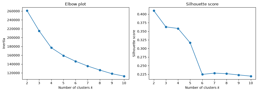

Loading...

The silhouette score is highest at $k=2$. That is not an artefact: the deepest split in the data really is the myeloid/lymphoid division we saw along PC1, and a criterion that rewards well-separated compact clusters will find it. But a partition into two groups is a poor description of blood, where we know a handful of cell types are present. The score stays above 0.3 up to $k=5$ and then falls sharply, from 0.32 to 0.22, between $k=5$ and $k=6$, after which it is flat. The elbow plot bends in the same region: the reduction in inertia is large up to $k=4$–5 and modest thereafter. We therefore take $k=5$, the largest number of clusters that the data still supports well.

This tension is worth dwelling on. Clustering criteria measure geometric separation, whereas we are interested in biological categories, and the two need not agree. The criteria narrow the range of sensible choices; they do not make the choice for us.

k-means with five clusters¶

kmeans = KMeans(n_clusters=5, n_init=10, random_state=0).fit(Y)
labels = kmeans.labels_
pd.Series(labels).value_counts().sort_index().rename("cells per cluster")

We plot the clusters in the plane of the first two principal components, which we know from the single-cell PCA chapter carries most of the lineage information.

pc = pd.DataFrame(scores[:, :3], columns=["PC1", "PC2", "PC3"])
pc["cluster"] = labels.astype(str)

fig, axes = plt.subplots(1, 2, figsize=(13, 5))
sns.scatterplot(data=pc, x="PC1", y="PC2", hue="cluster", palette="Set2", s=10, ax=axes[0])
sns.scatterplot(data=pc, x="PC2", y="PC3", hue="cluster", palette="Set2", s=10, ax=axes[1])
for ax in axes:
    ax.legend(title="Cluster", markerscale=2)
plt.tight_layout()
plt.show()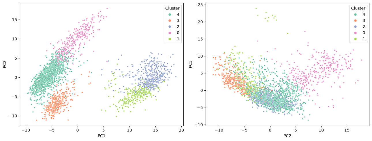

The clusters occupy contiguous, largely non-overlapping regions, which is reassuring but not by itself evidence that they are biologically meaningful — k-means would have produced five contiguous Voronoi cells even from a structureless cloud of points. To decide whether these clusters are real we need the marker genes.

Annotating the clusters with marker genes¶

We now compute, for each cluster, the mean log expression of a panel of established PBMC markers. Note that these genes play no part in the clustering itself beyond whatever weight they happened to receive as highly variable genes; the annotation is an external check.

marker_panel = {
    "CD3D":   "T cell (pan)",
    "CD3E":   "T cell (pan)",
    "IL7R":   "CD4 T cell",
    "CCR7":   "naive T cell",
    "CD8A":   "CD8 T cell",
    "NKG7":   "cytotoxic granule",
    "GNLY":   "NK cell",
    "MS4A1":  "B cell",
    "CD79A":  "B cell",
    "LYZ":    "monocyte",
    "CD14":   "classical monocyte",
    "S100A8": "classical monocyte",
    "FCGR3A": "CD16+ monocyte / NK",
    "MS4A7":  "CD16+ monocyte",
    "FCER1A": "dendritic cell",
    "PPBP":   "platelet",
}
markers = list(marker_panel)

mean_expression = expression_df[markers].groupby(labels).mean()
mean_expression.index.name = "cluster"
mean_expression.round(2)

The same table is easier to read as a heatmap. We standardise each gene across clusters, so that the colour shows in which cluster a gene is relatively high rather than how strongly it is expressed overall.

zscored = (mean_expression - mean_expression.mean()) / mean_expression.std()

plt.figure(figsize=(11, 4))
sns.heatmap(zscored, cmap="vlag", center=0, annot=mean_expression.round(1),
            fmt="", cbar_kws={"label": "z-score across clusters"})
plt.xlabel("Marker gene")
plt.ylabel("Cluster")
plt.title("Mean log expression per cluster (numbers), z-scored (colour)")
plt.tight_layout()
plt.show()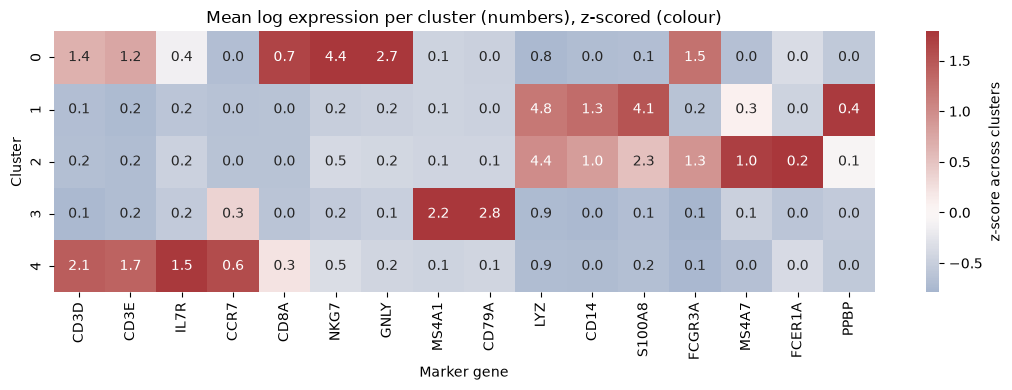

The pattern is unambiguous, and each cluster is defined by a coherent set of markers rather than by a single gene:

annotation = {
    0: "NK and cytotoxic T cells",
    1: "CD14+ classical monocytes",
    2: "CD16+ monocytes and dendritic cells",
    3: "B cells",
    4: "CD4 T cells",
}
summary = pd.DataFrame({
    "cell type": pd.Series(annotation),
    "cells": pd.Series(labels).value_counts().sort_index(),
})
summary["fraction"] = (summary["cells"] / summary["cells"].sum()).map("{:.1%}".format)
summary.index.name = "cluster"
summary

• Cluster 4 is the largest and expresses CD3D, CD3E and IL7R but no cytotoxic genes: these are helper (CD4) T cells.

• Cluster 0 expresses NKG7 and GNLY strongly together with FCGR3A, and only moderate CD3D: a mixture of NK cells and cytotoxic CD8 T cells.

• Cluster 3 expresses MS4A1 and CD79A and nothing else in the panel: B cells.

• Clusters 1 and 2 both express LYZ at high levels and are therefore both monocytic, but they differ sharply in a second marker: cluster 1 has high CD14 and S100A8 (classical monocytes) whereas cluster 2 has high FCGR3A and MS4A7 (non-classical, CD16+ monocytes) and also carries the FCER1A-positive dendritic cells.

The clusters therefore correspond, one to one, to recognisable immune cell populations. Importantly, the proportions are plausible too: T cells are by far the most abundant PBMC population, followed by monocytes, B cells and NK cells, which is what we see.

What the clustering missed¶

Platelets, marked by PPBP, are not given a cluster of their own at $k=5$; most of them end up inside the classical monocyte cluster, which is why cluster 1 shows the highest mean PPBP in the heatmap above. The FCER1A-positive dendritic cells fare similarly: they are clearly enriched in cluster 2, but only enough to nudge its mean.

rare = pd.DataFrame({
    "PPBP+ (platelet)": expression_df["PPBP"] > 2,
    "FCER1A+ (dendritic)": expression_df["FCER1A"] > 1,
}).groupby(labels).sum()
rare["cluster size"] = pd.Series(labels).value_counts().sort_index()
rare.index.name = "cluster"
rare

Both populations amount to a few dozen cells out of 2,638. k-means minimises a total sum of squares, and a cluster of thirty cells removes far less of that sum than splitting a population of six hundred, so small populations are systematically absorbed into larger ones. Detecting rare cell types requires either a much larger $k$ — at the price of fragmenting the abundant types — or methods that do not optimise a global variance criterion. This is a real and well-known limitation, not a peculiarity of this dataset.

A Gaussian mixture model of the same cells¶

k-means assigns every cell to exactly one cluster and, as discussed in the theory chapter, implicitly assumes clusters of similar spherical extent. Cell populations are not equally tight — a population of activated cells is more heterogeneous than a population of resting ones — so it is natural to fit a Gaussian mixture model instead, letting each component have its own variance along each principal component.

from sklearn.mixture import GaussianMixture

gmm = GaussianMixture(n_components=5, covariance_type="diag",
                      random_state=0, n_init=5).fit(Y)
gmm_labels = gmm.predict(Y)
gmm_means = expression_df[markers].groupby(gmm_labels).mean()
gmm_means.index.name = "component"
gmm_means.round(2)

The mixture model draws its boundaries differently. It merges the two monocyte clusters that k-means kept apart, and instead splits the T cells in two — one component with high CCR7 and no cytotoxic genes, the other with lower CCR7 and a trace of NKG7, which corresponds to the classical distinction between naive and memory/effector T cells. A cross-tabulation shows where the two solutions agree and where they do not.

pd.crosstab(pd.Series(labels, name="k-means"),
            pd.Series(gmm_labels, name="GMM component"))

The cross-tabulation also reveals something the marker table alone would not. The mixture model’s cytotoxic component is broad: besides taking over most of the k-means NK cluster (281 of its 310 cells), it absorbs cells from every other cluster, including 97 of the 264 cells in k-means cluster 1, so that almost half of its 522 cells come from the other k-means clusters. That is a direct consequence of letting components have their own variances. A component fitted to a genuinely dispersed population acquires a large covariance, and a large covariance makes it the most probable origin for any cell that lies far from all the tight components. k-means, which treats every cluster as having the same spherical extent, cannot behave this way — the flip side of the drawback noted in the theory chapter.

Neither partition is “correct”. Both are valid five-way divisions of a population that actually contains more than five biologically distinct types; which division an algorithm prefers depends on its assumptions about cluster shape. Presented with the same data, a working immunologist would use several such views side by side.

The advantage of a mixture model is that it is a soft clustering: instead of an assignment it gives the responsibility $\gamma_{nk}$, the posterior probability that cell $n$ belongs to component $k$. Cells whose largest responsibility is far from one lie in the overlap between components, and their assignment should not be taken at face value.

responsibilities = gmm.predict_proba(Y)
confidence = responsibilities.max(axis=1)

fig, axes = plt.subplots(1, 2, figsize=(12, 4.5))
sns.histplot(confidence, bins=40, ax=axes[0])
axes[0].set(xlabel="Largest responsibility $\\max_k \\gamma_{nk}$", ylabel="Cells")
sc = axes[1].scatter(scores[:, 0], scores[:, 1], c=confidence, cmap="magma", s=6)
axes[1].set(xlabel="PC1", ylabel="PC2", title="Assignment confidence")
fig.colorbar(sc, ax=axes[1], label="max responsibility")
plt.tight_layout()
plt.show()

print(f"{(confidence < 0.9).mean():.1%} of cells are assigned with probability below 0.9")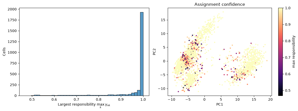

12.8% of cells are assigned with probability below 0.9

The great majority of cells are assigned with near-certainty. The uncertain ones sit along the interfaces between components. Within the lymphoid cloud at low PC1, the split between the two T cell components and the transition towards the cytotoxic cells are both gradual rather than sharp. In the myeloid cloud at high PC1, the uncertain cells lie mostly in its lower left part, and they are torn between the monocyte component and the broad cytotoxic component: the large-covariance effect described above.

Discussion¶

Clustering pbmc3k works remarkably well, and it is worth being clear about why, because the reasons do not carry over to every dataset.

We had a ground truth. The decisive step in this chapter was not running k-means, which took a fraction of a second, but the marker-gene table that let us name the clusters. Peripheral blood is among the best-characterised tissues in biology, and each of our clusters could be matched to a cell type that immunologists had defined long before single-cell sequencing existed. In a less well-characterised tissue there may be no such marker panel, and a cluster can then only be interpreted through the genes that distinguish it from the others.

The groups were genuinely discrete. A monocyte and a B cell are separate cell types with separate transcriptional programmes, and nothing lies between them; our clusters are therefore separated by empty space. Where cells vary continuously, as they do along a differentiation trajectory, a clustering imposes boundaries on what is really a continuum. Even within our own data we saw a hint of this at the T cell/NK boundary, where the mixture model’s responsibilities became uncertain.

Every cell was measured the same way. All 2,638 cells come from one donor, one library and one sequencing run, so there are no batch effects to be mistaken for biology. Had we combined donors, the first principal component might well have separated donors rather than cell types.

In routine single-cell analysis, the problems we ran into, from the choice of $k$ to the rare populations and the disagreement between algorithms, are handled by clustering at several resolutions and annotating each of them, rather than by searching for one true value of $k$. Clustering is exploratory rather than confirmatory: the algorithm proposes a partition, and the marker genes decide whether it means anything.