PCA of single cells

Introduction¶

In the PCA chapter we developed principal component analysis as a decomposition of an expression matrix $\mathbf{X} \approx \mathbf{U}\mathbf{S}\mathbf{V}^{\textsf{T}}$ into gene-specific effects $\mathbf{u}^{(i)}$ and sample-specific effects $\mathbf{v}^{(i)}$. Here we put that machinery to work on a single-cell RNA sequencing (scRNA-seq) dataset.

The shift from bulk to single-cell data changes the meaning of a “sample” in an instructive way. In a bulk experiment, one column of $\mathbf{X}$ is a tissue biopsy — a mixture of thousands of cells of many different types, and the measured expression is an average over that mixture. In a single-cell experiment, one column is a single cell, and the dominant source of variation is simply which type of cell we happened to capture. This turns out to make PCA far easier to interpret: we will see that the leading principal components correspond, quite directly, to the major immune cell lineages.

We use the classic pbmc3k dataset from 10x Genomics: approximately 2,700 peripheral blood mononuclear cells (PBMCs) from a single healthy donor, sequenced on the 10x Chromium platform. PBMCs are the white blood cells of the immune system — T cells, B cells, natural killer (NK) cells, monocytes and dendritic cells — and they are an ideal teaching set because the cell types present are known in advance and each of them has well-established marker genes.

This chapter prepares the ground for the chapter Cluster analysis of single cells, where we cluster the same cells with the methods from the clustering chapter. Both notebooks are self-contained, so the loading and preprocessing code below is repeated there.

Retrieving the data¶

The data is distributed by 10x Genomics as a gzipped tar archive of about 7 MB containing three files in the Matrix Market sparse format:

• matrix.mtx — the counts, one line per non-zero entry,

• genes.tsv — the Ensembl identifier and symbol of each of the 32,738 genes,

• barcodes.tsv — the cell barcode of each of the 2,700 cells.

We download the archive once and cache it locally, exactly as we do for the TCGA sets elsewhere in this book.

# When the page runs in the browser (JupyterLite), we install seaborn, and fetch the data from a copy in the book's
# repository, as the 10x Genomics server does not allow downloads from within a browser
import sys
if sys.platform == "emscripten":
    import os
    import micropip
    await micropip.install(["seaborn", "pyodide-http"])
    import pyodide_http
    pyodide_http.patch_all()
    from urllib.request import urlretrieve
    archive = "../data/pbmc3k_filtered_gene_bc_matrices.tar.gz"
    os.makedirs("../data", exist_ok=True)
    if not os.path.exists(archive):
        urlretrieve("https://raw.githubusercontent.com/statisticalbiotechnology/dsbook/main/dsbook/unsupervised/data/"
                    "pbmc3k_filtered_gene_bc_matrices.tar.gz", archive)
    # scipy's Matrix Market reader starts several threads, which the browser does not support
    import scipy.io._fast_matrix_market
    scipy.io._fast_matrix_market.PARALLELISM = 1

import os
import sys
import tarfile
import requests
import numpy as np
import pandas as pd
import matplotlib.pyplot as plt
import seaborn as sns
from scipy.io import mmread

IN_COLAB = 'google.colab' in sys.modules
data_dir = "data/" if IN_COLAB else "../data/"
os.makedirs(data_dir, exist_ok=True)

url = "https://cf.10xgenomics.com/samples/cell-exp/1.1.0/pbmc3k/pbmc3k_filtered_gene_bc_matrices.tar.gz"
archive = os.path.join(data_dir, "pbmc3k_filtered_gene_bc_matrices.tar.gz")
matrix_dir = os.path.join(data_dir, "filtered_gene_bc_matrices", "hg19")

if not os.path.exists(matrix_dir):
    if not os.path.exists(archive):
        print("Downloading pbmc3k ...")
        response = requests.get(url, stream=True)
        response.raise_for_status()
        with open(archive, "wb") as handle:
            for chunk in response.iter_content(chunk_size=1 << 16):
                handle.write(chunk)
    with tarfile.open(archive, "r:gz") as tar:
        tar.extractall(path=data_dir, filter="data")
print("Matrix directory:", matrix_dir)

Downloading pbmc3k ...

Matrix directory: ../data/filtered_gene_bc_matrices/hg19

The Matrix Market file is read with scipy.io.mmread. It is stored as genes $\times$ cells, and we transpose it so that the rows of our matrix are cells and the columns are genes. This is the orientation scikit-learn expects: observations in rows, features in columns.

counts = mmread(os.path.join(matrix_dir, "matrix.mtx")).T.tocsr()   # cells x genes
genes = pd.read_csv(os.path.join(matrix_dir, "genes.tsv"), sep="\t",
                    header=None, names=["ensembl", "symbol"])
barcodes = pd.read_csv(os.path.join(matrix_dir, "barcodes.tsv"), sep="\t",
                       header=None, names=["barcode"])
gene_names = genes["symbol"].to_numpy(dtype=str)

print(f"{counts.shape[0]} cells x {counts.shape[1]} genes")
print(f"{counts.nnz / np.prod(counts.shape):.1%} of the entries are non-zero")

2700 cells x 32738 genes
2.6% of the entries are non-zero

Note how empty the matrix is: fewer than 3% of all gene–cell combinations are non-zero. This sparsity is the defining technical feature of scRNA-seq data. A single cell contains only a few hundred thousand mRNA molecules, of which we sequence a small fraction, so a gene expressed at a modest level simply may not be observed at all in a given cell. Keeping the matrix in a sparse format is what makes it possible to handle these data on a laptop.

Quality control¶

Not every barcode corresponds to a healthy cell. Two summary statistics per cell catch most of the problems:

1. The number of genes detected. Very low values indicate an empty droplet or a broken cell whose mRNA has leaked out; very high values often indicate a doublet, i.e. two cells that ended up in the same droplet.

2. The fraction of counts from mitochondrial genes (the genes whose symbol starts with MT-). A dying cell loses its cytoplasmic mRNA through the ruptured membrane, while the mitochondrially encoded transcripts stay behind, so a high mitochondrial fraction is a signature of a stressed or dying cell.

total_counts = np.asarray(counts.sum(axis=1)).ravel()
n_genes = np.asarray((counts > 0).sum(axis=1)).ravel()
is_mito = np.char.startswith(gene_names, "MT-")
mito_fraction = np.asarray(counts[:, is_mito].sum(axis=1)).ravel() / total_counts

qc = pd.DataFrame({"total_counts": total_counts,
                   "n_genes": n_genes,
                   "mito_fraction": mito_fraction})

fig, axes = plt.subplots(1, 3, figsize=(13, 3.5))
sns.histplot(qc["total_counts"], bins=50, ax=axes[0]).set(xlabel="Counts per cell")
sns.histplot(qc["n_genes"], bins=50, ax=axes[1]).set(xlabel="Genes detected per cell")
sns.scatterplot(data=qc, x="total_counts", y="mito_fraction", s=6, ax=axes[2]).set(
    xlabel="Counts per cell", ylabel="Mitochondrial fraction")
plt.tight_layout()
plt.show()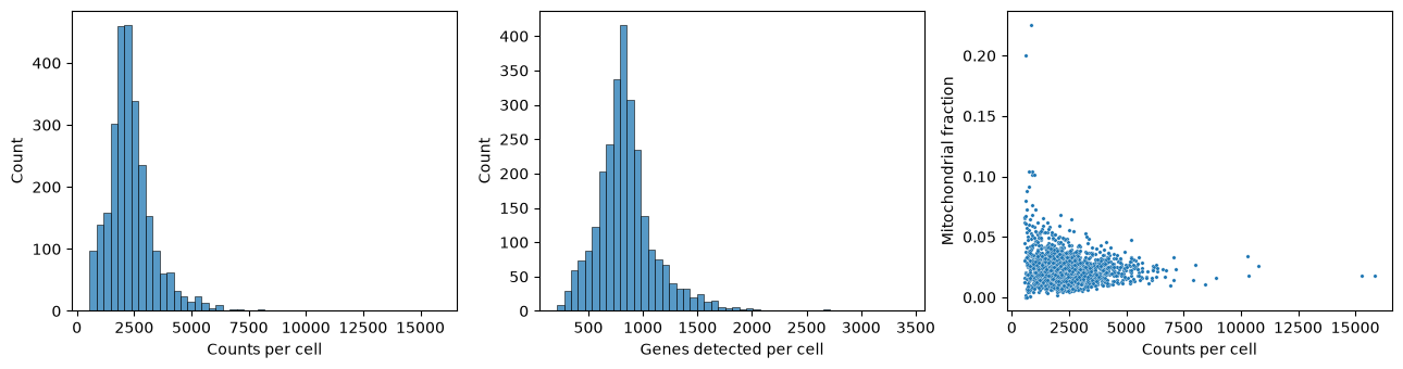

The distributions are unimodal and well behaved, which is expected for a dataset that 10x Genomics has already filtered for cell-containing droplets. We nevertheless apply the customary thresholds: keep cells with between 200 and 2,500 detected genes and less than 5% mitochondrial counts. We also drop genes seen in fewer than three cells, since such genes carry essentially no information about cell-to-cell structure but would add thousands of near-empty columns.

keep_cells = (n_genes > 200) & (n_genes < 2500) & (mito_fraction < 0.05)
counts = counts[keep_cells]
total_counts = total_counts[keep_cells]

keep_genes = np.asarray((counts > 0).sum(axis=0)).ravel() >= 3
counts = counts[:, keep_genes]
gene_names = gene_names[keep_genes]

print(f"After filtering: {counts.shape[0]} cells x {counts.shape[1]} genes")

After filtering: 2638 cells x 13656 genes

Normalisation and feature selection¶

Cells differ several-fold in how many mRNA molecules were captured from them. This is largely technical, a matter of how efficiently each droplet captured and converted its mRNA, although cell types also differ in their mRNA content. We therefore divide each cell by its total count and multiply by 10⁴, so that every cell is expressed as counts per ten thousand. As in the bulk chapters we then take a logarithm, here $\log(1+x)$ so that the many zeros remain finite:

where $C_{cg}$ is the raw count of gene $g$ in cell $c$.

expression = counts.multiply(1e4 / total_counts[:, None]).tocsr().log1p()
expression = np.asarray(expression.todense())
expression_df = pd.DataFrame(expression, columns=gene_names)

We are left with about 13,700 genes, but the great majority of them are either expressed at a uniform level in every cell or so rarely detected that what we observe is mostly sampling noise. We therefore select the 1,000 genes with the highest variance across cells. These highly variable genes are the ones that can possibly distinguish cell types from one another. This is a simplified version of standard practice: single-cell packages such as Seurat and Scanpy rank genes by a variance that is corrected for each gene’s mean expression, because the raw variance favours highly expressed genes.

Finally we standardise each selected gene to zero mean and unit variance. Without this step, PCA on log-expression would be dominated by a handful of extremely highly expressed genes; standardisation puts a weakly and a strongly expressed marker on the same footing. We clip the standardised values at $\pm 10$ so that a single cell with an extreme outlier count cannot single-handedly define a principal component. In this dataset no value is that extreme, so the clipping is only a safeguard.

variances = expression.var(axis=0)
hvg_index = np.argsort(variances)[::-1][:1000]
hvg_names = gene_names[hvg_index]

X = expression[:, hvg_index]
X = (X - X.mean(axis=0)) / X.std(axis=0)
X = np.clip(X, -10, 10)

print("Ten most variable genes:", ", ".join(hvg_names[:10]))
print("Matrix for PCA:", X.shape)

Ten most variable genes: LYZ, S100A9, HLA-DRA, CST3, TYROBP, S100A8, NKG7, LGALS1, CD74, CCL5
Matrix for PCA: (2638, 1000)

Several of the most variable genes are immediately recognisable: LYZ and S100A9 are monocyte genes, NKG7 is a cytotoxic granule gene of NK and CD8 T cells, and CD74 and HLA-DRA are antigen-presentation genes of B cells and monocytes. The feature selection has, without being told anything about cell types, picked out genes that differ between cell types.

Principal component analysis¶

We now run PCA, using scikit-learn as in the theory chapter. We ask for 50 components, far more than we intend to interpret, so that we can look at how quickly the explained variance decays.

from sklearn.decomposition import PCA

pca = PCA(n_components=50, random_state=0)
scores = pca.fit_transform(X)      # cells x components
loadings = pca.components_         # components x genes
print("Scores:", scores.shape, " Loadings:", loadings.shape)

Scores: (2638, 50)  Loadings: (50, 1000)

It is worth pausing on how this maps onto the notation of the PCA chapter. There we wrote $\mathbf{X} = \mathbf{U}\mathbf{S}\mathbf{V}^{\textsf{T}}$ for a genes $\times$ samples matrix, with $\mathbf{U}$ holding the gene-specific effects and $\mathbf{V}$ the sample-specific effects. Our matrix here is transposed — cells in rows, genes in columns — so the roles swap over: pca.components_ contains the gene-specific vectors $\mathbf{u}^{(i)}$, one row per component, and pca.fit_transform returns the cell-specific scores, which are the entries of $\mathbf{v}^{(i)}$ scaled by the singular value $S_i$. The quantity $R^2_i = S_i^2 / \sum_j S_j^2$ of the PCA chapter is what scikit-learn calls explained_variance_ratio_.

How much variance does each component explain?¶

evr = pca.explained_variance_ratio_

fig, axes = plt.subplots(1, 2, figsize=(11, 4))
axes[0].plot(range(1, 51), 100 * evr, "o-", ms=4)
axes[0].set(xlabel="Principal component", ylabel="Explained variance (%)",
            title="Scree plot")
axes[1].plot(range(1, 51), 100 * np.cumsum(evr), "o-", ms=4)
axes[1].set(xlabel="Number of components", ylabel="Cumulative explained variance (%)",
            title="Cumulative explained variance")
plt.tight_layout()
plt.show()

print(f"PC1 explains {100*evr[0]:.1f}% of the variance")
print(f"The first 15 components explain {100*evr[:15].sum():.1f}%")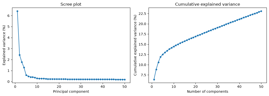

PC1 explains 6.4% of the variance
The first 15 components explain 15.8%

The numbers look disappointing at first sight: the first component explains only about 6% of the variance and the first fifteen together less than a fifth of it. The reason is not that single-cell data has little structure — it is that single-cell data has vastly more noise. Each gene in each cell is sampled from a small pool of molecules, so a large share of the total variance is Poisson counting noise which, being independent between genes, spreads itself thinly and evenly over all 1,000 dimensions. The biological signal is concentrated in a handful of components; the noise is not concentrated anywhere.

The scree plot makes this visible. There is a clear break after the first four or five components, followed by a long, almost flat tail. Components beyond roughly the tenth are, for practical purposes, indistinguishable from each other in magnitude — the hallmark of noise.

What do the first components mean?¶

The gene-specific vector $\mathbf{u}^{(i)}$ tells us which genes drive component $i$. Genes with a large positive loading are high in cells with a positive score, and genes with a large negative loading are high in cells with a negative score.

for i in range(4):
    order = np.argsort(loadings[i])
    print(f"PC{i+1} ({100*evr[i]:.1f}%)")
    print("   positive:", ", ".join(hvg_names[order[::-1][:8]]))
    print("   negative:", ", ".join(hvg_names[order[:8]]))

PC1 (6.4%)
   positive: CST3, TYROBP, FCER1G, LST1, FTL, AIF1, FTH1, LGALS1
   negative: RPS27A, RPL21, RPS3A, RPL9, RPSA, LTB, RPS25, RPL31
PC2 (2.4%)
   positive: NKG7, CST7, GZMA, PRF1, GZMB, CTSW, FGFBP2, HLA-C
   negative: HLA-DRA, CD79A, MS4A1, TCL1A, HLA-DQB1, HLA-DQA1, HLA-DRB1, HLA-DMA
PC3 (1.8%)
   positive: GZMB, NKG7, CST7, FGFBP2, GZMA, PRF1, CCL5, GNLY
   negative: VIM, JUNB, RPS10, RPL36A, LDHB, RPLP0, RPL36, RPS25
PC4 (1.3%)
   positive: HLA-DQA1, CD79A, CD79B, HLA-DQB1, MS4A1, CD74, HLA-DPB1, HLA-DPA1
   negative: CD3D, S100A8, S100A6, S100A4, CD3E, IL32, S100A9, IL7R

Each component reads as a contrast between two groups of cells:

• PC1 opposes CST3, TYROBP, FCER1G, LST1 and AIF1 — all genes of the myeloid lineage, i.e. monocytes and dendritic cells — to a block of ribosomal protein genes and LTB, which are characteristic of small resting lymphocytes. PC1 is the myeloid/lymphoid axis, the deepest division in the blood.

• PC2 opposes the cytotoxic granule machinery NKG7, GZMA, GZMB, PRF1 and FGFBP2 of NK cells to CD79A, MS4A1, TCL1A and the HLA-D class II genes of B cells.

• PC3 again picks out cytotoxic genes, this time against a background of housekeeping and ribosomal genes.

• PC4 separates the B cell programme (CD79A, CD79B, MS4A1, class II) from the T cell and monocyte programme (CD3D, CD3E, IL7R, S100A8, S100A9).

Note that a single cell type can appear on several components, and that a single component can involve more than one cell type. Principal components are constrained to be orthogonal to one another, which is a geometric requirement, not a biological one; there is no reason for the axes of maximum variance to line up one-to-one with cell types.

The cells in principal component space¶

We now project the cells onto their first components and colour them by the expression of established marker genes. This is the single most informative plot in the chapter: if the components capture cell identity, then cells expressing the same marker should occupy the same region.

markers = {
    "CD3D":   "T cells",
    "IL7R":   "CD4 T cells",
    "NKG7":   "NK / cytotoxic cells",
    "LYZ":    "Monocytes",
    "FCGR3A": "CD16+ monocytes / NK",
    "MS4A1":  "B cells",
}

pc = pd.DataFrame(scores[:, :3], columns=["PC1", "PC2", "PC3"])

fig, axes = plt.subplots(2, 3, figsize=(14, 8), sharex=True, sharey=True)
for ax, (gene, label) in zip(axes.flat, markers.items()):
    sc = ax.scatter(pc["PC1"], pc["PC2"], c=expression_df[gene],
                    cmap="viridis", s=4)
    ax.set_title(f"{gene} — {label}")
    ax.set_xlabel("PC1")
    ax.set_ylabel("PC2")
    fig.colorbar(sc, ax=ax, shrink=0.8, label="log expression")
plt.tight_layout()
plt.show()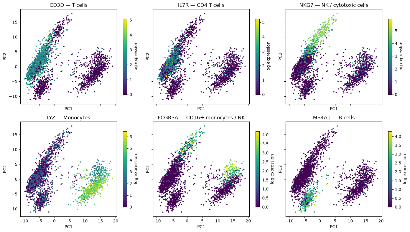

The plot separates the major lineages cleanly. The cells at high PC1 are the LYZ-positive monocytes; the cells at low PC1 are the lymphocytes, and within them high PC2 marks the NKG7-positive cytotoxic cells while low PC2 marks the MS4A1-positive B cells. CD3D-positive T cells occupy the large intermediate lobe.

FCGR3A is a useful reminder that markers are not exclusive: it is expressed both by NK cells and by the non-classical (CD16+) subset of monocytes, and accordingly it lights up in two separate places in the plot. Cell identity is established by combinations of markers, not by single genes.

The cytotoxic arm is worth a closer look, because it is the one place in this dataset where the cell types shade into each other. Plotting PC2 against PC3 resolves it into a gradient:

fig, axes = plt.subplots(1, 2, figsize=(12, 4.5))
for ax, gene in zip(axes, ["CD3D", "NKG7"]):
    sc = ax.scatter(pc["PC2"], pc["PC3"], c=expression_df[gene], cmap="viridis", s=4)
    ax.set(xlabel="PC2", ylabel="PC3", title=gene)
    fig.colorbar(sc, ax=ax, shrink=0.85, label="log expression")
plt.tight_layout()
plt.show()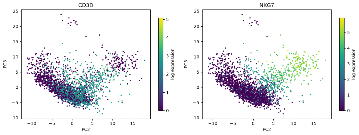

Both PC2 and PC3 increase with NKG7, so the cytotoxic cells form a diagonal arm reaching away from the main body of lymphocytes. Along that arm the CD3D signal fades: the cells nearest the main body are cytotoxic T cells, which carry both the T cell receptor and the granule genes, whereas the cells at the tip have lost CD3D altogether and are NK cells. There is no gap between them — this is a genuine biological continuum, and it is the one place in this dataset where drawing a boundary will be a matter of judgement rather than of reading off an obvious gap. The small island of ten cells at the top of both panels, at PC3 above 20, is a different population, the platelets, which we return to below.

The correlation between each marker and each component quantifies the same thing:

marker_list = ["CD3D", "IL7R", "LYZ", "CD14", "FCGR3A", "MS4A1", "CD79A", "NKG7", "GNLY", "PPBP"]
corr = pd.DataFrame(
    {f"PC{j+1}": [np.corrcoef(scores[:, j], expression_df[g])[0, 1] for g in marker_list]
     for j in range(4)},
    index=marker_list)

sns.heatmap(corr, cmap="vlag", center=0, annot=True, fmt=".2f",
            cbar_kws={"label": "Pearson correlation"})
plt.title("Marker genes vs. principal components")
plt.show()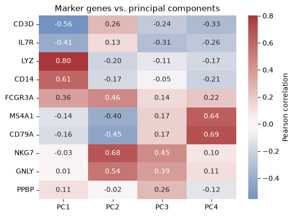

LYZ and CD14 correlate strongly and positively with PC1, CD3D and IL7R negatively; NKG7 and GNLY load on PC2 and PC3; MS4A1 and CD79A load on PC4 and negatively on PC2. PPBP, a platelet gene, reaches no more than 0.26 with any of the four. Platelets make up only about 1% of these cells, and a population that small contributes too little variance to define any of the leading components. They are not invisible, though: ten of them form the island at the top of the PC2–PC3 plot, because they have very low levels of the ribosomal and housekeeping transcripts on the negative side of PC3. They stand out on PC3 only as a side effect, while the component itself is defined by the cytotoxic genes. This is a general and important limitation: PCA finds abundant structure, not necessarily interesting structure.

Why reduce dimensions before clustering?¶

The plots above already tell us that the cells fall into groups, and in the chapter Cluster analysis of single cells we will find those groups formally. It is worth being explicit about why we will cluster in the space of the first 10–20 principal components rather than in the original 1,000-dimensional gene space.

1. Noise reduction. As the scree plot showed, the biological signal is concentrated in the leading components while the counting noise is spread over all of them. Truncating the decomposition after 15 components discards most of the noise and retains most of the signal, so distances between cells become much more reliable.

2. The curse of dimensionality. Clustering algorithms such as k-means depend on Euclidean distances. In high dimensions, the distances between all pairs of points become increasingly similar, and the contrast that a clustering algorithm needs in order to distinguish “near” from “far” is washed out.

3. Computation. k-means and Gaussian mixture models on $2{,}638 \times 15$ numbers are instantaneous; on $2{,}638 \times 1{,}000$ they are not, and a full covariance matrix in 1,000 dimensions has about half a million free parameters, far too many to estimate from a cluster of a few hundred cells.

4. Visualisation. Two or three components can be plotted directly, which lets us sanity-check a clustering by eye — something we will do repeatedly in the single-cell clustering chapter.

PCA does have one limitation here: it is linear. It rotates and translates the data, but it cannot unfold a curved structure. For the coarse cell types in this dataset that is not a problem, as the marker plots show. For finer structure, such as a continuum of differentiating cells, more elaborate methods are usually applied on top of the principal components.