Multiple Regression Example

In mass spectrometry-based proteomics, the peptides of a sample are separated by liquid chromatography before they enter the mass spectrometer. The peptides are pumped through a column packed with a hydrophobic material, in a solvent that slowly becomes less polar. Each peptide sticks to the column until the solvent is apolar enough to release it, so it leaves the column, or elutes, at a characteristic retention time. Hydrophobic peptides stick harder and elute later. Being able to predict a peptide’s retention time helps identify it: if a peptide that we think we have identified elutes far from its predicted time, the identification is probably wrong.

In this example, we predict the retention time of a peptide from its amino-acid composition. Already in 1980, Meek showed that a peptide’s retention time can be approximated by a sum of contributions from its amino acids,

where $n_a$ is the number of times amino acid $a$ occurs in the peptide, and $\beta_a$ is the retention coefficient of that amino acid. This is a multiple regression with 20 predictors, one per amino acid. We fit it with a ridge penalty, test it on peptides that were not used for the fit, and look at what the fitted coefficients tell us about the amino acids.

Data Loading and Preparation¶

We use a set of about 14,000 peptides, without modifications, whose retention times were measured on the same chromatography setup. The data come with the retention-time predictor DeepLC. The file lists each peptide’s sequence and its observed retention time in seconds, which we convert to minutes.

# When the page runs in the browser (JupyterLite), we install seaborn, and let Python download files through the browser
import sys
if sys.platform == "emscripten":
    import micropip
    await micropip.install(["seaborn", "pyodide-http"])
    import pyodide_http
    pyodide_http.patch_all()

import os
import urllib.request

import numpy as np
import pandas as pd

# Cache the downloaded table, so that we only fetch it once
data_dir = "../data" if os.path.isdir("../data") else "data"
os.makedirs(data_dir, exist_ok=True)
local_file = os.path.join(data_dir, "deeplc_unmod.csv")
if not os.path.exists(local_file):
    url = "https://raw.githubusercontent.com/compomics/DeepLC/ddde602795635873af5dbfbba234fc896f09ea4c/examples/datasets/unmod.peprec"
    urllib.request.urlretrieve(url, local_file)

peptides = pd.read_csv(local_file)
# One retention time in the file is malformed; we turn it into a missing value and drop it
peptides["rt"] = pd.to_numeric(peptides["observed_retention_time"], errors="coerce") / 60
peptides = peptides.dropna(subset=["rt"])[["peptide", "rt"]]
peptides

For each peptide we count how often each of the 20 amino acids occurs. These counts are our predictors.

amino_acids = list("ACDEFGHIKLMNPQRSTVWY")
counts = pd.DataFrame({aa: peptides["peptide"].str.count(aa) for aa in amino_acids}, index=peptides.index)
counts.head()

Most peptides end with K or R, as they were produced by digesting proteins with trypsin, which cuts after these two amino acids. Other amino acids are rare: W, for instance, occurs in only about one peptide in ten.

Training and Test Set¶

To find out how well the model predicts the retention time of peptides it has not seen, we randomly set aside 30% of the peptides as a test set. We fit the model to the remaining 70%, the training set, and only use the test set to evaluate the predictions.

X = counts.to_numpy(dtype=float)
y = peptides["rt"].to_numpy()

rng = np.random.default_rng(1)
shuffled = rng.permutation(len(y))
n_train = int(0.7 * len(y))
train, test = shuffled[:n_train], shuffled[n_train:]
print(f"{len(train)} training peptides and {len(test)} test peptides")

9985 training peptides and 4280 test peptides

Fitting the Model with a Ridge Loss¶

We minimize the ridge loss with scipy.optimize.minimize, just as in the regularization chapter. The intercept, the last element of beta, is left out of the penalty, so that the fit does not depend on the average retention time.

When the predictors are measured in different units, such as protein levels and age, we standardize them first, so that the penalty treats them alike. Here all predictors are counts of amino acids, so we keep them as they are. We can then read each coefficient directly as the number of minutes that one residue of that amino acid adds to the retention time.

from scipy.optimize import minimize

# Define the Ridge loss function
def ridge_loss(beta, X, y, lambda_ridge):
    # Prediction
    y_pred = X @ beta[:-1] + beta[-1]  # Last beta is intercept
    # Ridge loss: Sum of Squared Errors + penalty on the coefficients (not on the intercept)
    error = y - y_pred
    loss = np.sum(error ** 2) + lambda_ridge * np.sum(beta[:-1] ** 2)
    return loss

# Fit a model by minimizing the ridge loss, starting from all parameters set to zero
def fit_ridge(X, y, lambda_ridge):
    initial_beta = np.zeros(X.shape[1] + 1)
    return minimize(ridge_loss, initial_beta, args=(X, y, lambda_ridge), method='L-BFGS-B').x

beta = fit_ridge(X[train], y[train], lambda_ridge=1)
coefficients = pd.Series(beta[:-1], index=amino_acids)
intercept = beta[-1]
print(f"Intercept: {intercept:.1f} minutes")

Intercept: 47.1 minutes

With about 10,000 training peptides and only 21 parameters, the penalty hardly changes the fit; we return to the penalty at the end of the chapter.

The Retention Coefficients¶

Each coefficient tells how many minutes one more residue of that amino acid adds to the predicted retention time, when the counts of all other amino acids are kept the same.

import matplotlib.pyplot as plt
import seaborn as sns

sorted_coefficients = coefficients.sort_values()
plt.figure(figsize=(8, 5))
plt.bar(sorted_coefficients.index, sorted_coefficients.values,
        color=np.where(sorted_coefficients.values > 0, "tab:orange", "tab:blue"))
plt.axhline(0, color="black", linewidth=0.8)
plt.xlabel("Amino acid")
plt.ylabel("Retention coefficient (minutes per residue)")
plt.show()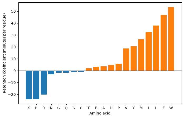

The coefficients follow the chemistry of the amino acids. The largest positive coefficients belong to amino acids with large hydrophobic side chains: W, F, L, I and M, followed by Y and V. Each such residue makes the peptide stick harder to the column. The negative coefficients belong to K, R and H, which carry a positive charge in the acidic solvent used for the separation. A charged residue keeps the peptide in the polar solvent, so it elutes earlier. The remaining amino acids are small or polar, and contribute little. Without being told anything about chemistry, the regression has recovered a hydrophobicity scale of the amino acids.

Predicted vs Observed Retention Time¶

We now predict the retention times of the test peptides and compare them with the observed ones. As a single measure of fit we use the coefficient of determination,

the fraction of the variation in the observed values $y_i$ that the predictions $\hat{y}_i$ explain. A perfect model has $R^2 = 1$, and a model that always predicts the average $\bar{y}$ has $R^2 = 0$.

def r_squared(y, y_pred):
    return 1 - np.sum((y - y_pred) ** 2) / np.sum((y - y.mean()) ** 2)

y_pred = X @ coefficients.to_numpy() + intercept
print(f"R^2 on the training set: {r_squared(y[train], y_pred[train]):.2f}")
print(f"R^2 on the test set:     {r_squared(y[test], y_pred[test]):.2f}")
print(f"Median absolute error on the test set: {np.median(np.abs(y[test] - y_pred[test])):.0f} minutes")

plt.figure(figsize=(7, 6))
plt.scatter(y[test], y_pred[test], s=4, alpha=0.3)
plt.plot([y.min(), y.max()], [y.min(), y.max()], color='red', linestyle='--', linewidth=2)
plt.xlabel('Observed retention time (minutes)')
plt.ylabel('Predicted retention time (minutes)')
plt.title('Test peptides')
plt.show()

R^2 on the training set: 0.87
R^2 on the test set:     0.88
Median absolute error on the test set: 13 minutes

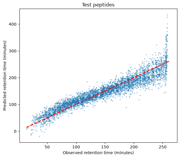
The dashed red line marks perfect predictions. The amino-acid composition explains most of the variation in retention time, and the model does about as well on the test peptides as on the training peptides, so it has not overfitted. Still, half of the test peptides are predicted more than 13 minutes from their observed retention time. The composition ignores the order of the amino acids, and so their neighbors and the peptide’s structure, which also affect the retention. Modern predictors, such as DeepLC, use the full sequence and are considerably more accurate.

Near the end of the run, at about 255 minutes, the points form a vertical stripe. These are most likely very hydrophobic peptides that stay on the column until the end of the separation, when the column is flushed with apolar solvent and they all elute at once. A sum of contributions from the amino acids has no such ceiling, so the model predicts ever later retention times for them. Such a pattern in a plot of predicted against observed values is a sign that the relation between predictors and response is not linear over the whole range.

When the Training Set Is Small¶

The ridge penalty pays off when there are few training examples per parameter. To see this, we repeatedly draw 25 random peptides from the training set, fit the model to them with different values of $\lambda$, and measure $R^2$ on the test set. With only 25 peptides to determine 21 parameters, the fit is poorly determined. A rare amino acid such as W occurs in just a few of the peptides, if any, so its coefficient rests on very few observations.

lambdas = [0.1, 0.3, 1, 3, 10, 30, 100]
n_small, n_draws = 25, 50

test_r2 = {lambda_ridge: [] for lambda_ridge in [0] + lambdas}
for draw in range(n_draws):
    small = rng.choice(train, n_small, replace=False)
    for lambda_ridge in test_r2:
        beta = fit_ridge(X[small], y[small], lambda_ridge)
        test_r2[lambda_ridge].append(r_squared(y[test], X[test] @ beta[:-1] + beta[-1]))

median_r2 = {lambda_ridge: np.median(r2) for lambda_ridge, r2 in test_r2.items()}
plt.figure(figsize=(7, 5))
plt.plot(lambdas, [median_r2[l] for l in lambdas], marker="o", label="Ridge")
plt.axhline(median_r2[0], color="gray", linestyle="--", label=r"No penalty ($\lambda = 0$)")
plt.xscale("log")
plt.xlabel(r"$\lambda$")
plt.ylabel(r"Median $R^2$ on the test set")
plt.title(f"Models fitted to {n_small} peptides")
plt.legend()
plt.show()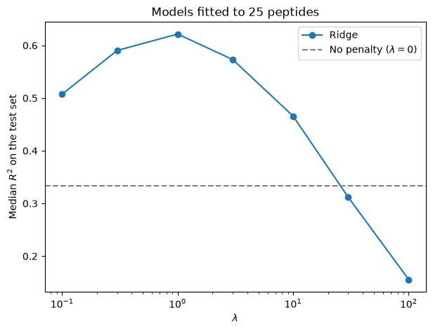

A moderate penalty gives better predictions for new peptides than no penalty, as it keeps the poorly determined coefficients from taking extreme values. Too strong a penalty, however, shrinks all coefficients towards zero, and the predictions approach the average retention time. Here we used the test set to compare the values of $\lambda$; the validation chapter shows how to choose $\lambda$ from the training data alone.